Backpropagation Explained Step by Step, with NumPy Code

Say you are sending money to a cousin in Germany. Your bank converts rupees to dollars, and a second service converts dollars to euros. If 1 rupee buys 0.012 dollars and 1 dollar buys 0.92 euros, how many euros does one extra rupee add at the far end?

You do not need the whole route at once. You multiply the two local rates: 0.012 × 0.92 = 0.011 euros per rupee. Add a third conversion and you multiply one more rate.

That is the chain rule, and backpropagation is nothing more than this multiplication, done carefully for every weight in a network. In the XOR network from scratch you used two backprop lines without deriving them. Here you will derive them, check them numerically and see how frameworks automate the job.

What is backpropagation?

Map the money transfer to a network:

• Each conversion step is one operation in the network: a multiply, an add, an activation, the loss.
• Each exchange rate is a local derivative: how much that step's output moves when its input moves a little.
• The final "euros per rupee" is the gradient of the loss with respect to one weight.
• Working from the euro end back to the rupee end is the backward pass.

Backpropagation is an algorithm that computes the gradient of a neural network's loss with respect to every parameter by applying the chain rule from the output back to the inputs, reusing intermediate values stored during the forward pass.

Backprop only computes gradients. Changing the weights is a separate job done by an optimiser such as SGD or Adam, covered in gradient descent and optimizers.

The chain rule on a computational graph

Any network can be drawn as a computational graph: nodes are simple operations, and arrows carry numbers between them. The forward pass flows left to right. The backward pass flows right to left, and each node multiplies the gradient arriving from its right by its own local derivative.

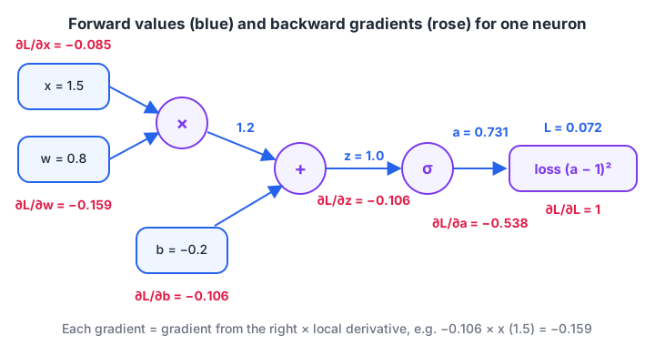
One neuron as a graph. Blue numbers are forward values; rose numbers are gradients of the loss, each one the gradient from the right times the local derivative.

A single neuron, by hand

Take one input x = 1.5, weight w = 0.8, bias b = −0.2, a sigmoid and a squared-error loss against target y = 1. The forward pass is z = w·x + b, then a = σ(z), then L = (a − y)².

Backward, one local rate at a time:

1. dL/da = 2(a − y), the slope of the loss.
2. da/dz = a(1 − a), the slope of the sigmoid.
3. dz/dw = x and dz/db = 1, the slopes of the weighted sum.
4. Multiply along each path: dL/dw = dL/da · da/dz · x and dL/db = dL/da · da/dz · 1.

import math

x, w, b, y = 1.5, 0.8, -0.2, 1.0
z = w * x + b                     # forward
a = 1 / (1 + math.exp(-z))
L = (a - y) ** 2

dL_da = 2 * (a - y)               # backward: local rates
da_dz = a * (1 - a)
dL_dw = dL_da * da_dz * x
dL_db = dL_da * da_dz * 1
print(f"z={z:.3f} a={a:.4f} L={L:.5f}")
print(f"dL/dw={dL_dw:.5f}  dL/db={dL_db:.5f}")

def loss(w_, b_):                 # nudge w and measure, to check
    a_ = 1 / (1 + math.exp(-(w_ * x + b_)))
    return (a_ - y) ** 2
eps = 1e-6
print(f"numeric dL/dw={(loss(w + eps, b) - loss(w - eps, b)) / (2 * eps):.5f}")

Both ways give the same number, about −0.159. The negative sign says "raise w to reduce the loss", which makes sense because the output 0.731 is below the target of 1.

Backpropagation through a tiny network with matrices

A real layer has many neurons, so the scalar rules become matrix rules. Three patterns cover a fully connected network:

The last row is worth noticing. With cross-entropy loss instead of squared error, the sigmoid's a(1 − a) cancels out, leaving the clean error A − Y. That is one reason classifiers use cross-entropy.

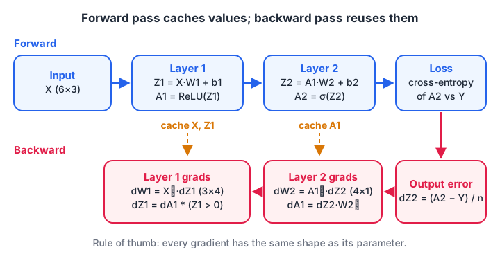
The forward pass saves each layer's input and pre-activation. The backward pass uses exactly those saved values, layer by layer, to build every gradient.

Here is a 3-4-1 network with ReLU in the hidden layer, trained for one step on a mini-batch of six rows. The function returns every gradient so you can inspect or test them.

import numpy as np
rng = np.random.default_rng(3)

X = rng.normal(size=(6, 3))                       # 6 samples, 3 features
Y = np.array([[1], [0], [1], [1], [0], [0]], float)
P = {"W1": rng.normal(scale=0.5, size=(3, 4)), "b1": np.zeros(4),
     "W2": rng.normal(scale=0.5, size=(4, 1)), "b2": np.zeros(1)}

def forward_backward(P, X, Y):
    Z1 = X @ P["W1"] + P["b1"];  A1 = np.maximum(0, Z1)
    Z2 = A1 @ P["W2"] + P["b2"]; A2 = 1 / (1 + np.exp(-Z2))
    n = len(X)
    loss = -np.mean(Y * np.log(A2) + (1 - Y) * np.log(1 - A2))
    dZ2 = (A2 - Y) / n                            # sigmoid + cross-entropy
    g = {"W2": A1.T @ dZ2, "b2": dZ2.sum(axis=0)}
    dA1 = dZ2 @ P["W2"].T
    dZ1 = dA1 * (Z1 > 0)                          # ReLU derivative
    g["W1"], g["b1"] = X.T @ dZ1, dZ1.sum(axis=0)
    return loss, g

loss, g = forward_backward(P, X, Y)
print(f"loss = {loss:.4f}")
for k, v in g.items():
    print(k, "grad shape", v.shape, "matches param:", v.shape == P[k].shape)

A quick sanity rule: every gradient has exactly the same shape as its parameter. If dW1 comes out as (4, 3) when W1 is (3, 4), you have a missing transpose.

Gradient checking: how to trust your gradients

A wrong gradient rarely crashes your code. The loss just falls slowly, or not at all, and you waste hours tuning the learning rate. A gradient check catches this in seconds.

The idea: for each parameter, nudge it up by a tiny ε, then down by ε, and measure the change in loss. The centred difference (L(θ+ε) − L(θ−ε)) / 2ε approximates the true gradient. Compare it with backprop using the relative error |a − b| / (|a| + |b|).

import numpy as np
rng = np.random.default_rng(3)
X = rng.normal(size=(6, 3)); Y = np.array([[1], [0], [1], [1], [0], [0]], float)
P = {"W1": rng.normal(scale=0.5, size=(3, 4)), "b1": np.zeros(4),
     "W2": rng.normal(scale=0.5, size=(4, 1)), "b2": np.zeros(1)}

def forward_backward(P):
    Z1 = X @ P["W1"] + P["b1"]; A1 = np.tanh(Z1)          # tanh: smooth, no kinks
    A2 = 1 / (1 + np.exp(-(A1 @ P["W2"] + P["b2"])))
    loss = -np.mean(Y * np.log(A2) + (1 - Y) * np.log(1 - A2))
    dZ2 = (A2 - Y) / len(X)
    dZ1 = (dZ2 @ P["W2"].T) * (1 - A1 ** 2)
    return loss, {"W2": A1.T @ dZ2, "b2": dZ2.sum(0), "W1": X.T @ dZ1, "b1": dZ1.sum(0)}

_, grads = forward_backward(P)
eps = 1e-5
for name, theta in P.items():
    num = np.zeros_like(theta)
    for i in np.ndindex(theta.shape):
        old = theta[i]
        theta[i] = old + eps; up, _ = forward_backward(P)
        theta[i] = old - eps; down, _ = forward_backward(P)
        theta[i] = old
        num[i] = (up - down) / (2 * eps)
    rel = np.abs(num - grads[name]).max() / (np.abs(num).max() + np.abs(grads[name]).max())
    print(f"{name}: relative error {rel:.2e}", "OK" if rel < 1e-6 else "CHECK THIS")

Relative errors near 1e-9 mean the gradients are right. Around 1e-3 or larger means a bug. This check uses tanh instead of ReLU on purpose: ReLU's corner at zero can fool the numerical estimate when a value sits right on it.

Why not always use numerical gradients?

Because they are slow. The check above needs two forward passes per parameter. This tiny network has 21 parameters, so 42 passes. A model with 10 million weights would need 20 million passes for one update. Backprop gets all of them from one forward and one backward pass. Use numerical gradients only as a test.

Autograd: how frameworks do backprop for you

PyTorch and TensorFlow record every operation in the forward pass, build the graph automatically, and run the chain rule when you ask. This is reverse-mode automatic differentiation. You can build a toy version in plain Python to see that nothing magical is involved:

import math

class Value:
    def __init__(self, data, parents=(), local=()):
        self.data, self.grad, self.parents, self.local = data, 0.0, parents, local
    def __add__(self, o): return Value(self.data + o.data, (self, o), (1.0, 1.0))
    def __mul__(self, o): return Value(self.data * o.data, (self, o), (o.data, self.data))
    def sigmoid(self):
        s = 1 / (1 + math.exp(-self.data))
        return Value(s, (self,), (s * (1 - s),))
    def backward(self, upstream=1.0):            # chain rule: upstream x local rate
        self.grad += upstream
        for parent, rate in zip(self.parents, self.local):
            parent.backward(upstream * rate)

x, w, b = Value(1.5), Value(0.8), Value(-0.2)
a = (w * x + b).sigmoid()
err = a + Value(-1.0)
loss = err * err
loss.backward()
print(f"loss = {loss.data:.5f}")
print(f"dL/dw = {w.grad:.5f}, dL/db = {b.grad:.5f}, dL/dx = {x.grad:.5f}")

It reproduces the hand-computed −0.159 for w. Real frameworks walk the graph in topological order instead of recursing, work on whole tensors and run on GPUs, but the bookkeeping is the same. In PyTorch 2.x the same neuron looks like this:

import torch

x = torch.tensor(1.5)
w = torch.tensor(0.8, requires_grad=True)
b = torch.tensor(-0.2, requires_grad=True)
loss = (torch.sigmoid(w * x + b) - 1.0) ** 2
loss.backward()                  # fills w.grad and b.grad
print(w.grad, b.grad)            # tensor(-0.1586) tensor(-0.1058)

# For your own custom layers, PyTorch can gradient-check them too
# (inputs must be double precision):
from torch.autograd import gradcheck
inp = torch.randn(4, 3, dtype=torch.double, requires_grad=True)
print(gradcheck(torch.tanh, (inp,), eps=1e-6, atol=1e-4))

Practising this derivation with a mentor is the fastest way to stop fearing it. A machine learning course in Indore that teaches backprop by hand before frameworks is what Debugshala runs at Old Palasia.

Common backpropagation mistakes

• Forgetting to zero gradients. In PyTorch, .grad accumulates. Call optimizer.zero_grad() every step, or gradients from old batches pile up.
• Missing the 1/n from the mean. Your gradients become n times too large, which looks like a learning-rate problem.
• Using the activated value where the pre-activation belongs. ReLU's derivative needs Z1 > 0, not A1. Here they agree, but for other activations they do not.
• Shape mismatches hidden by broadcasting. NumPy may silently broadcast (6,) against (6, 1) into (6, 6). Keep targets as column vectors.
• Skipping the gradient check. Ten lines of checking saves an afternoon of guessing.

Deep stacks also bring vanishing and exploding gradients, which come from multiplying many local rates; activation functions explains the cause and the cure.

Key takeaways

• Backprop multiplies local derivatives along the graph, from the loss back to each weight.
• The forward pass must cache inputs and pre-activations for the backward pass.
• For a dense layer: dW = A_prev.T @ dZ and dA_prev = dZ @ W.T; gradients match parameter shapes.
• Sigmoid with cross-entropy gives the simple output error A − Y.
• Check hand-written gradients numerically with a relative error below about 1e-6.

For more drills on derivatives and NumPy shapes, attempt calculus-flavoured coding quizzes on Debugshala Test.