

RNN and LSTM Explained: Recurrent Neural Networks in NumPy
RNN and LSTM explained with NumPy cell steps: hidden state, backpropagation through time, vanishing gradients, LSTM gates, GRU and a PyTorch forecaster.
Ride an iBus along the BRTS corridor from Niranjanpur to Rajiv Gandhi Square and watch the conductor. At every stop she updates one number in her head: passengers on board. She does not recount the whole bus. She takes the previous count, adds the people who boarded and subtracts those who left.
Now the depot asks whether a ticket checker boarded forty stops ago. Her running count cannot say; it was overwritten long ago. So she keeps a small notebook, writes down only what matters and crosses out what no longer does.
The running count is the hidden state of a recurrent neural network. The notebook, with its rules for writing and erasing, is the cell state of an LSTM.
What is a recurrent neural network?
Map the bus to the model:
- Each stop is one time step
tin the sequence. - The boarding and leaving numbers are the input
x_t. - The count in her head is the hidden state
h_t. - Her rule "old count plus change" is the recurrent cell, the same rule at every stop.
A recurrent neural network is a neural network for sequential data that applies the same cell at each time step, combining the current input with a hidden state carried over from the previous step, so its output depends on everything it has seen so far.
The networks earlier in this series, from neural network from scratch to CNNs, take fixed-size inputs. A sentence or a sensor stream has variable length, and order matters. RNNs handle both.
The RNN cell step
One step computes h_t = tanh(Wx · x_t + Wh · h_(t−1) + b). Wx reads the new input, Wh reads the memory, and tanh keeps values between −1 and 1. Unrolling the loop over time gives the picture below.
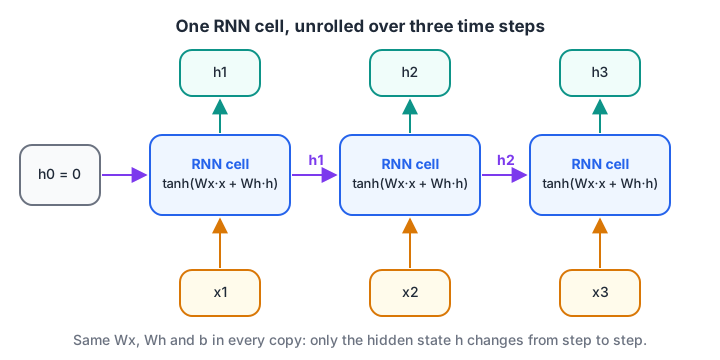
An RNN unrolled over three time steps. It is one cell, drawn three times: the weights Wx and Wh are shared, and only the hidden state changes.
import numpy as np
rng = np.random.default_rng(0)

input_size, hidden_size = 2, 4
Wx = rng.normal(scale=0.5, size=(hidden_size, input_size))   # input -> hidden
Wh = rng.normal(scale=0.5, size=(hidden_size, hidden_size))  # hidden -> hidden (memory)
b = np.zeros(hidden_size)

def rnn_step(x_t, h_prev):
    return np.tanh(Wx @ x_t + Wh @ h_prev + b)

# 5 bus stops: (people boarding, people leaving), scaled to 0-1
sequence = np.array([[0.8, 0.0], [0.5, 0.1], [0.0, 0.6], [0.3, 0.3], [0.0, 0.0]])
h = np.zeros(hidden_size)                                    # empty memory at the start
for t, x_t in enumerate(sequence, start=1):
    h = rnn_step(x_t, h)                                     # same weights every step
    print(f"step {t}: input {x_t}  ->  hidden {np.round(h, 3)}")
print("parameters:", Wx.size + Wh.size + b.size, "(same count for 5 steps or 5,000)")
The hidden state changes at every stop, even at step 5 where the input is zero, because memory alone drives it. The 28 parameters do not grow with sequence length: weight sharing over time, as a CNN shares over space.
How RNNs are trained: backpropagation through time
To train an RNN, you unroll it over the whole sequence and run ordinary backpropagation through the unrolled graph. This is called backpropagation through time (BPTT). The gradient for Wh is summed over every step. Long sequences are cut into chunks, which is truncated BPTT.
Quick check
Why does an RNN have the same number of parameters for a 10-step and a 1,000-step sequence?
Weight sharing over time means one set of Wx, Wh and b is applied at every step.
Why do RNNs forget? The vanishing gradient through time
To learn that step 3 affects the output at step 50, the gradient must travel back 47 steps. At each step it is multiplied by the tanh slope and by Wh. If those factors are usually below 1, the gradient shrinks exponentially; if above 1, it explodes.
import numpy as np
rng = np.random.default_rng(2)

H = 16
Wx = rng.normal(scale=0.5, size=(H, 1))
Wh = rng.normal(scale=0.9 / np.sqrt(H), size=(H, H))
xs = rng.normal(size=(60, 1))                      # a 60-step input sequence

h, J = np.zeros(H), np.eye(H)                      # J = d h_t / d h_0
for t, x_t in enumerate(xs, start=1):
    h = np.tanh(Wx @ x_t + Wh @ h)
    J = np.diag(1 - h ** 2) @ Wh @ J               # chain rule through one more step
    if t in (1, 5, 10, 20, 40, 60):
        print(f"gradient reaching {t:2d} steps back: {np.linalg.norm(J):.2e}")
After 20 steps the gradient has fallen by about 100 times, and after 60 steps by about 2 million. The network effectively cannot learn dependencies that far apart. This is the same multiplication problem described in activation functions, only stretched across time instead of layers.
Exploding gradients have a simple fix, gradient clipping: rescale the gradient when its norm passes a threshold such as 1.0. Vanishing gradients need a new architecture.
What is an LSTM and how does it remember?
An LSTM adds a second memory, the cell state c_t, which works like the conductor's notebook. Three gates, each a sigmoid layer producing values between 0 and 1, control it:
- The forget gate
fdecides how much of the old notebook to keep. 1 means keep everything, 0 means erase. - The input gate
idecides how much of the new candidate informationgto write. - The cell updates by addition:
c_t = f · c_(t−1) + i · g. - The output gate
odecides how much of the notebook to reveal as the hidden state:h_t = o · tanh(c_t).
An LSTM is a recurrent neural network cell that keeps a separate cell state and uses learned forget, input and output gates to control what is erased, written and exposed at each step, which lets it learn dependencies across long sequences.
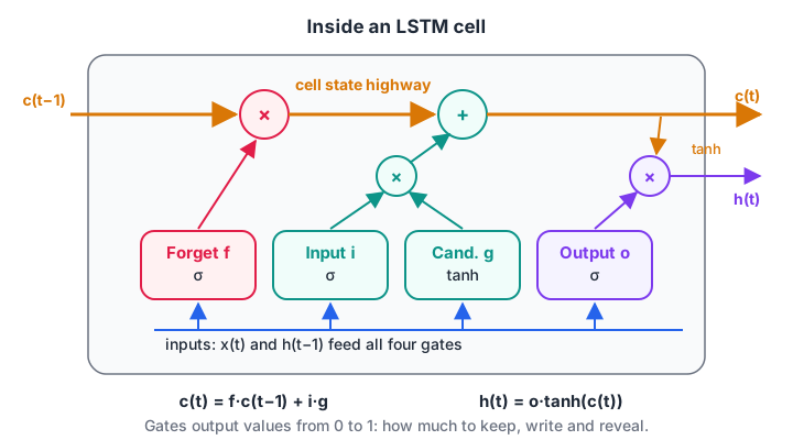
Inside an LSTM cell. The cell state runs along the top like a highway, changed only by a multiply (forget) and an add (write), so information and gradients can pass many steps with little loss.
The key is step 3. Because the cell state is updated by addition, the gradient flowing back along it is multiplied only by the forget gate. When something is worth remembering, the network learns to push that gate close to 1.
Here is a full LSTM step in NumPy. The forget-gate bias is set to 3 to imitate a gate that has learned "keep this", and the loop tracks how much gradient survives along the cell path:
import numpy as np
rng = np.random.default_rng(1)
sigmoid = lambda z: 1 / (1 + np.exp(-z))

H, D = 8, 1
W = {g: rng.normal(scale=0.3, size=(H, D + H)) for g in "figo"}
b = {"f": np.full(H, 3.0), "i": np.zeros(H), "g": np.zeros(H), "o": np.zeros(H)}

def lstm_step(x_t, h_prev, c_prev):
    z = np.concatenate([x_t, h_prev])               # input and previous output together
    f = sigmoid(W["f"] @ z + b["f"])                # forget gate: keep old memory?
    i = sigmoid(W["i"] @ z + b["i"])                # input gate: write new info?
    g = np.tanh(W["g"] @ z + b["g"])                # candidate info to write
    o = sigmoid(W["o"] @ z + b["o"])                # output gate: reveal memory?
    c = f * c_prev + i * g                          # cell state update (addition!)
    h = o * np.tanh(c)
    return h, c, f

h, c, keep = np.zeros(H), np.zeros(H), np.ones(H)   # keep = d c_t / d c_0 along the cell path
for t, x_t in enumerate(rng.normal(size=(60, 1)), start=1):
    h, c, f = lstm_step(x_t, h, c)
    keep *= f
    if t in (1, 5, 10, 20, 40, 60):
        print(f"step {t:2d}: forget gate mean {f.mean():.2f}, cell-path gradient {keep.mean():.2e}")
After 60 steps, about 6% of the gradient still survives along the cell path, compared with roughly two millionths in the plain RNN.
LSTM vs GRU vs plain RNN
| Plain RNN | LSTM | GRU | |
|---|---|---|---|
| Memory | Hidden state only | Hidden state + cell state | Hidden state only |
| Gates | None | Forget, input, output | Update, reset |
| Weight matrices per layer | 1 set | 4 sets | 3 sets |
| Long-range memory | Weak | Strong | Strong |
| Speed | Fastest | Slowest | In between |
| Good for | Very short sequences | Long sequences, default choice | When LSTM is too slow or data is small |
The GRU (gated recurrent unit) merges the forget and input gates into one update gate and drops the separate cell state. It often matches an LSTM with fewer parameters.
Quick check
Which LSTM gate decides how much of the previous cell state to keep?
The forget gate multiplies the old cell state; values near 1 keep it and values near 0 erase it.
Building an LSTM in PyTorch
This PyTorch 2.x model reads a window of past values, for example 30 days of a shop's sales, and predicts the next day:
import torch
from torch import nn

class SalesForecaster(nn.Module):
    def __init__(self, hidden_size=32):
        super().__init__()
        self.lstm = nn.LSTM(input_size=1, hidden_size=hidden_size,
                            num_layers=1, batch_first=True)
        self.head = nn.Linear(hidden_size, 1)

    def forward(self, x):                 # x: (batch, 30 days, 1 feature)
        out, (h_n, c_n) = self.lstm(x)    # out: (batch, 30, hidden_size)
        return self.head(out[:, -1, :])   # use the last step's hidden state

model = SalesForecaster()
pred = model(torch.randn(16, 30, 1))      # (16, 1)

# inside the training loop, after loss.backward():
torch.nn.utils.clip_grad_norm_(model.parameters(), max_norm=1.0)
Note batch_first=True: without it, PyTorch expects (sequence, batch, features). Swap nn.LSTM for nn.GRU and the forward pass returns out, h_n with no cell state. In Keras 3, keras.layers.LSTM(32) returns only the last hidden state by default; add return_sequences=True to get every step.
For forecasting work, compare any LSTM against simple baselines first, as covered in time series analysis basics. Sequence models are part of Debugshala's full Data Science & AI curriculum, while Debugshala's machine learning classes covering sequence models go deeper into training them.
RNNs and LSTMs vs transformers
RNNs read one step at a time, so training cannot run positions in parallel, and very long contexts still fade. Transformers use attention to let every position look at every other position at once, which is why large language models use them. The full story is in transformers and attention explained.
Common mistakes with RNNs and LSTMs
- Mixing up tensor layouts. Check
batch_firstin PyTorch; a swapped batch and time axis trains without error but learns nothing useful. - Skipping gradient clipping. RNN gradients can explode suddenly and turn the loss into
nan. - Unscaled inputs. Sales in rupees (thousands) next to percentages wrecks the tanh and sigmoid gates. Standardise each feature.
- Leaking the future. Build validation windows strictly after the training period.
Key takeaways
- An RNN updates a hidden state at every step with shared weights, so it handles any sequence length.
- Backpropagation through time multiplies one factor per step, so plain RNN gradients vanish or explode.
- An LSTM's additive cell state and learned gates keep both information and gradients alive.
- GRUs are a lighter gated alternative; clip gradients for any recurrent model.
- Transformers have replaced RNNs for large text models, but LSTMs still fit small and streaming tasks.
Next, autoencoders use networks like these to compress data without labels. To keep loops and state updates sharp, work through sequence and loop quizzes on Debugshala Test.
FAQ
What is the difference between RNN and LSTM?
An RNN keeps one hidden state updated by a single tanh layer, so it forgets quickly. An LSTM adds a separate cell state and three gates that control forgetting, writing and output, which keeps gradients alive so it learns long-range patterns plain RNNs miss.
Is LSTM still used in 2026?
Yes, though less for language. LSTMs and GRUs are still used for time series forecasting, sensor streams, speech on small devices and problems with little data. For large text tasks, transformers are standard because they train in parallel and scale better.
What is the vanishing gradient problem in RNNs?
It is the shrinking of the training signal as it travels back through many time steps. Each step multiplies the gradient by factors usually below 1, so after dozens of steps early inputs stop influencing learning. LSTMs and GRUs were designed to fix this.
What is the hidden state in an RNN?
The hidden state is a vector summarising everything the network has seen so far in the sequence. Each step computes it from the new input and the previous hidden state, and it feeds any output layer.
Where can I learn RNNs and LSTMs in Indore?
Debugshala teaches neural networks, including sequence models such as RNNs and LSTMs, in its Machine Learning and Data Science & AI courses in Indore. Classes are held at the Old Palasia campus in English and Hindi, and Data Science & AI is also available online. A free demo class is offered first.
From the team behind this site
Go further with the Data Science & AI Course at Debugshala
These tutorials are written by Debugshala, a training and placement institute at Old Palasia, Indore. The classroom course adds live mentoring, real projects and interview preparation.
- Offline classes at Old Palasia, Indore
- Free demo class before you pay
- Non-IT, fresher and year-gap friendly
- Placement assistance
700+ students placed · 200+ hiring partners · 4.9★ Google rating
