Convolutional Neural Networks (CNN) Explained with NumPy

A quality checker at a handloom unit in Maheshwar does not stare at a whole six-metre saree at once. She holds a small square card frame against the cloth and slides it along, row by row, looking for one specific fault: a broken thread, a slipped motif, a colour bleed.

She uses the same trained eye at every spot, because a broken thread looks the same near the border as in the middle. When she finds something, she marks its position on a small chart.

That sliding frame is a filter, her trained eye is the filter's weights, and the chart of marks is a feature map. A convolutional neural network runs dozens of these checkers at once, each hunting for a different pattern.

What is a convolutional neural network?

Map the handloom unit to a CNN:

• The saree is the input image, a grid of pixel values.
• The card frame is a small kernel (filter), often 3 × 3.
• Sliding it across the cloth is the convolution operation.
• Using the same eye everywhere is weight sharing.
• The chart of marks is the feature map that the next layer reads.

A convolutional neural network is a type of deep neural network that learns small filters and slides them across grid-shaped input, such as an image, so each layer detects local patterns and later layers combine them into larger shapes.

A plain network like the one in neural network from scratch connects every input to every neuron, with no notion that neighbouring pixels belong together. A CNN builds that notion in.

How does a convolution work?

Place the kernel on the top-left corner of the image. Multiply each kernel weight by the pixel under it, add the nine products, and write the sum into the first output cell. Slide one pixel right and repeat, row by row.

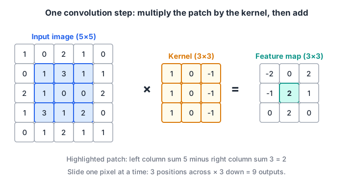
One step of a 2D convolution. The kernel's nine weights multiply the highlighted 3 × 3 patch, and the sum becomes a single cell of the 3 × 3 feature map.

Here is that operation in plain NumPy. The image is dark on the left and bright on the right, so it has one vertical edge. Two hand-made kernels look for vertical and horizontal edges:

import numpy as np

def conv2d(image, kernel, stride=1, padding=0):
    if padding:
        image = np.pad(image, padding)                 # zeros around the border
    kh, kw = kernel.shape
    oh = (image.shape[0] - kh) // stride + 1
    ow = (image.shape[1] - kw) // stride + 1
    out = np.zeros((oh, ow))
    for i in range(oh):
        for j in range(ow):
            patch = image[i * stride:i * stride + kh, j * stride:j * stride + kw]
            out[i, j] = np.sum(patch * kernel)         # multiply and add
    return out

image = np.array([[0, 0, 0, 9, 9, 9]] * 6, dtype=float)  # dark left, bright right
vertical_edge = np.array([[-1, 0, 1],
                          [-1, 0, 1],
                          [-1, 0, 1]], dtype=float)
horizontal_edge = vertical_edge.T

print("image:\n", image.astype(int))
print("vertical-edge feature map:\n", conv2d(image, vertical_edge).astype(int))
print("horizontal-edge feature map:\n", conv2d(image, horizontal_edge).astype(int))
print("stride 2, padding 1 shape:", conv2d(image, vertical_edge, stride=2, padding=1).shape)

The vertical-edge map lights up with 27 exactly where dark meets bright, and stays 0 on the flat regions. The horizontal-edge map is all zeros, because the image has no horizontal edges. In a real CNN, backpropagation learns the kernels, and first layers usually end up with edge detectors very like these.

Stride, padding and output size

Two settings control the output size:

• Stride is how far the kernel jumps each step. Stride 2 halves the width and height.
• Padding adds a border of zeros so the kernel can sit on edge pixels. Padding 1 with a 3 × 3 kernel keeps the size unchanged ("same" padding).

The output size for an input of size n, kernel k, padding p and stride s is (n + 2p − k) / s + 1, rounded down.

def conv_output_size(n, k, stride=1, padding=0):
    return (n + 2 * padding - k) // stride + 1

print("28x28, 3x3, no padding     ->", conv_output_size(28, 3))
print("28x28, 3x3, padding 1      ->", conv_output_size(28, 3, padding=1))
print("224x224, 7x7, stride 2, p3 ->", conv_output_size(224, 7, stride=2, padding=3))

h, w, c = 224, 224, 3                           # one colour photo
dense = (h * w * c) * 64 + 64                   # dense layer with 64 neurons
conv = (3 * 3 * c) * 64 + 64                    # conv layer with 64 filters of 3x3
print(f"dense layer weights: {dense:,}")
print(f"conv layer weights : {conv:,}  ({dense // conv:,}x fewer)")

A dense layer of 64 neurons on a colour photo needs about 9.6 million weights. A conv layer with 64 filters of size 3 × 3 × 3 needs 1,792. That saving, from weight sharing, is why CNNs made image recognition practical.

Channels: colour images and many filters

A colour image has three channels (red, green, blue), so each filter is really 3 × 3 × 3 and sums over all channels. A layer with 64 filters produces 64 feature maps, which become the 64 input channels of the next layer. In code, a conv weight tensor has shape (out_channels, in_channels, kernel_height, kernel_width).

What does pooling do in a CNN?

After a convolution, a pooling layer shrinks each feature map. Max pooling with a 2 × 2 window keeps the largest value in each tile; average pooling keeps the mean. Either way, a 4 × 4 map becomes 2 × 2.

import numpy as np

def pool2d(fmap, size=2, mode="max"):
    h, w = fmap.shape[0] // size, fmap.shape[1] // size
    blocks = fmap[:h * size, :w * size].reshape(h, size, w, size)  # split into tiles
    return blocks.max(axis=(1, 3)) if mode == "max" else blocks.mean(axis=(1, 3))

fmap = np.array([[1, 3, 0, 2],
                 [4, 8, 1, 0],
                 [0, 2, 9, 5],
                 [1, 1, 3, 7]], dtype=float)
print("max pool:\n", pool2d(fmap, 2, "max"))
print("average pool:\n", pool2d(fmap, 2, "avg"))

Pooling has no weights. It cuts later computation by four and adds some translation tolerance: if a strong edge moves one pixel but stays in the same tile, the max-pooled output does not change. Many modern networks use stride-2 convolutions instead.

CNN architecture: from pixels to prediction

A classic CNN stacks blocks of conv → ReLU → pool. Early blocks see small patches and detect edges.

Because each pooling step shrinks the map, later blocks see larger regions of the original image and combine edges into corners, textures, wheels or faces. Finally the maps are flattened into a vector and passed to dense layers that output class scores.

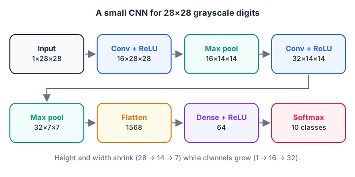
A small CNN for 28 × 28 grayscale digits. The spatial size shrinks while the number of channels grows, then a dense layer turns the features into 10 class probabilities.

The next block wires conv, ReLU and global max pooling into a tiny CNN that tells vertical bars from horizontal bars in noisy 8 × 8 images. It uses NumPy's sliding_window_view to do the convolution without Python loops, the same trick fast libraries use internally.

import numpy as np
from numpy.lib.stride_tricks import sliding_window_view
rng = np.random.default_rng(4)

def make_bar(kind):                                   # 8x8 image with one bar + noise
    img = rng.uniform(0, 0.3, size=(8, 8))
    k = rng.integers(1, 7)
    if kind == "vertical": img[:, k] += 1.0
    else:                  img[k, :] += 1.0
    return img

kernels = np.array([[[-1, 2, -1]] * 3,                # responds to vertical lines
                    np.array([[-1, 2, -1]] * 3).T])   # responds to horizontal lines

def tiny_cnn(img):
    patches = sliding_window_view(img, (3, 3))                 # (6, 6, 3, 3)
    fmaps = np.einsum("ijkl,ckl->cij", patches, kernels)       # conv: 2 feature maps
    fmaps = np.maximum(0, fmaps)                               # ReLU
    pooled = fmaps.max(axis=(1, 2))                            # global max pool
    return ["vertical", "horizontal"][pooled.argmax()], pooled

correct = 0
for t in range(200):
    kind = ["vertical", "horizontal"][t % 2]
    pred, scores = tiny_cnn(make_bar(kind))
    correct += pred == kind
print("example scores (vertical, horizontal):", np.round(scores, 2))
print(f"accuracy on 200 random bar images: {correct / 200:.0%}")

It scores 100% even though the bar can appear in any row or column. Weight sharing plus global pooling makes the network ask "is there a vertical line anywhere?", not "is there a line in column 3?".

Building a CNN in PyTorch

This PyTorch 2.x model matches the architecture diagram above. The comments track the tensor shape for a batch of 28 × 28 grayscale images:

import torch
from torch import nn

model = nn.Sequential(
    nn.Conv2d(in_channels=1, out_channels=16, kernel_size=3, padding=1),  # (N, 16, 28, 28)
    nn.BatchNorm2d(16),
    nn.ReLU(),
    nn.MaxPool2d(kernel_size=2),                                          # (N, 16, 14, 14)
    nn.Conv2d(16, 32, kernel_size=3, padding=1),                          # (N, 32, 14, 14)
    nn.ReLU(),
    nn.MaxPool2d(2),                                                      # (N, 32, 7, 7)
    nn.Flatten(),                                                         # (N, 1568)
    nn.Linear(32 * 7 * 7, 64),
    nn.ReLU(),
    nn.Dropout(0.3),
    nn.Linear(64, 10),                                                    # 10 class logits
)
x = torch.randn(8, 1, 28, 28)       # PyTorch uses (batch, channels, height, width)
print(model(x).shape)               # torch.Size([8, 10])

BatchNorm2d and Dropout are the layers from batch normalisation and dropout, now applied per channel. Train it with the AdamW loop from gradient descent and optimizers. In Keras 3 the equivalent layers are keras.layers.Conv2D(16, 3, padding="same", activation="relu") and keras.layers.MaxPooling2D(), and Keras expects channels last: (batch, height, width, channels).

For real projects with limited data, you rarely train a CNN from zero. You start from one pretrained on millions of images and adapt it, as explained in transfer learning. If you want to build image projects like this with mentor reviews, a hands-on deep learning track at Debugshala's Old Palasia campus is part of the Machine Learning course.

Common mistakes when building CNNs

• Wrong channel order. PyTorch wants (N, C, H, W) and Keras wants (N, H, W, C). A swapped image still runs but learns nonsense.
• Miscounting the flatten size. Compute it from the output-size formula, or run one dummy batch and print the shape.
• Skipping input normalisation. Pixel values of 0 to 255 make training unstable; scale to 0 to 1 or standardise per channel.
• Too much pooling on small images. Each 2 × 2 pool halves the size; a 28 × 28 image is down to 1 × 1 after five.
• No data augmentation. Flips, small rotations and crops are cheap extra training data and reduce overfitting sharply.

Key takeaways

• A convolution slides a small kernel over the image, multiplying and summing at each position.
• Weight sharing makes conv layers tiny and lets them detect a pattern anywhere.
• Stride and padding set the output size: (n + 2p − k) / s + 1.
• Pooling shrinks feature maps and adds tolerance to small shifts.
• Stacked conv blocks grow from edges to textures to objects, then dense layers classify.

Images are grids; text and time series are sequences, which is where RNNs and LSTMs come in. For more practice with grids and indices, solve array-indexing puzzles on Debugshala Test.