Neural Network from Scratch in NumPy: Train XOR Step by Step

Picture a new trainee at a tiffin service in Bhawarkuan. Every morning she has to decide whether a customer will reorder tomorrow. She looks at two things: did they finish the food, and did they reply to the feedback message? At first she guesses badly.

Each evening the manager tells her who actually reordered. She adjusts how much she trusts each clue. "Finishing the food matters more than I thought. The message reply matters less." After a few weeks, her guesses are good.

She never received a rulebook. She just kept making a guess, checking how wrong it was, and adjusting how much weight she gave each clue. That is exactly what a neural network does, only with numbers.

What a Neural Network Actually Is

Map the trainee to the vocabulary:

• The clues (finished food, replied to message) are inputs.
• How much she trusts each clue is a weight.
• Her general optimism before looking at clues is the bias.
• Turning her gut score into a "yes, 80% likely" is the activation function.
• How wrong she was each evening is the loss.
• Adjusting her trust after each evening is gradient descent.

A neural network is a function made of layers of neurons, where each neuron computes a weighted sum of its inputs plus a bias, passes it through a non-linear activation, and the weights are learned by repeatedly reducing a loss with gradient descent.

One neuron, by hand

A single neuron computes z = w1*x1 + w2*x2 + b, then applies an activation. The sigmoid activation squashes any number into the range 0 to 1, which is handy for probabilities.

import numpy as np

def sigmoid(z):
    return 1 / (1 + np.exp(-z))

x = np.array([1.0, 0.0])        # finished food = yes, replied = no
w = np.array([2.5, 0.8])        # trust in each clue
b = -1.0                        # bias

z = x @ w + b                   # weighted sum: 1*2.5 + 0*0.8 - 1.0
print("weighted sum z =", z)
print("sigmoid(z)     =", round(sigmoid(z), 3), "-> chance of reorder")
for z_val in [-4, -1, 0, 1, 4]:
    print(f"sigmoid({z_val:2d}) = {sigmoid(z_val):.3f}")

A big positive z gives a value near 1, a big negative z gives a value near 0, and zero gives exactly 0.5. Without this squashing step, stacking layers would collapse into one plain linear equation, and the network could never learn curved boundaries.

The Network Diagram: Layers, Weights and the Forward Pass

The network you will train has 2 inputs, a hidden layer of 4 neurons and 1 output neuron. Every input connects to every hidden neuron, and every hidden neuron connects to the output.

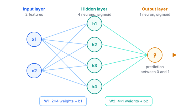
A 2-4-1 neural network: 8 weights from input to hidden, 4 weights from hidden to output, plus one bias per neuron, so 17 numbers to learn.

The forward pass is just matrix multiplication done layer by layer:

1. h = sigmoid(X @ W1 + b1): each hidden neuron mixes the two inputs its own way.
2. out = sigmoid(h @ W2 + b2): the output neuron mixes the four hidden signals.

If you have four training rows, X has shape (4, 2), W1 has shape (2, 4) and h comes out as (4, 4): one row per example, one column per hidden neuron. Writing it as matrices lets NumPy process every example at once instead of looping.

Loss and Gradient Descent

After the forward pass you need a single number that says how bad the predictions are. We will use mean squared error (MSE): the average of (prediction - target)². A perfect network has loss 0.

Gradient descent asks, for each weight, "if I increase this weight a little, does the loss go up or down?" That slope is the gradient. You then step the weight a small amount in the downhill direction. The step size is the learning rate.

Here is gradient descent on a single weight, so you can see the idea without any network around it:

# Find w so that prediction = w * x matches the data (true answer is w = 3)
xs = [1, 2, 3, 4]
ys = [3, 6, 9, 12]
w, lr = 0.0, 0.01

for step in range(41):
    preds = [w * x for x in xs]
    loss = sum((p - y) ** 2 for p, y in zip(preds, ys)) / len(xs)
    grad = sum(2 * (p - y) * x for p, y, x in zip(preds, ys, xs)) / len(xs)
    w -= lr * grad
    if step % 8 == 0:
        print(f"step {step:2d}  w = {w:.3f}  loss = {loss:.3f}")

The weight climbs from 0 towards 3 and the loss shrinks towards 0. A neural network does this for all 17 weights at the same time.

Backpropagation, Intuitively

The output neuron is easy: you can directly see how wrong it was. But how do you blame a hidden neuron that never saw the target?

Backpropagation passes the error backwards using the chain rule from calculus. Think of the tiffin manager tracing a complaint: the customer was unhappy (output error), the delivery was late (hidden cause), because the route was poor (earlier cause). Each link gets blame in proportion to how much it contributed.

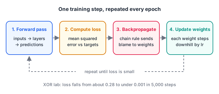
One training step. The forward pass makes predictions, the loss scores them, backprop assigns blame to every weight, and gradient descent updates them. Repeat thousands of times.

In code, backprop for our network is just two lines:

• d_out = (out - y) * out * (1 - out): error at the output, times the slope of the sigmoid there. (The sigmoid's slope is s * (1 - s), a neat property. The lab code also multiplies by 2 / n, which comes from averaging the squared error.)
• d_h = d_out @ W2.T * h * (1 - h): the output error sent back through the weights W2, times the slope of each hidden sigmoid.

Then the gradient for a weight matrix is "the input to that layer" times "the error at its output": h.T @ d_out for W2 and X.T @ d_h for W1.

Lab: Train a Neural Network on XOR in NumPy

XOR outputs 1 when exactly one of two inputs is 1. It is the classic test because no single straight line separates the 1s from the 0s, so a lone neuron cannot learn it. First, prove that to yourself:

import numpy as np

X = np.array([[0, 0], [0, 1], [1, 0], [1, 1]], dtype=float)
y = np.array([0, 1, 1, 0], dtype=float)

w, b, lr = np.zeros(2), 0.0, 1.0
for epoch in range(5000):                    # one neuron, no hidden layer
    out = 1 / (1 + np.exp(-(X @ w + b)))
    grad = (out - y) / len(X)
    w -= lr * X.T @ grad
    b -= lr * grad.sum()

print("single-neuron outputs:", np.round(out, 3))
print("predictions:", (out > 0.5).astype(int), "targets:", y.astype(int))

Every output sits at 0.5. The best a straight line can do is shrug. Now add a hidden layer of four neurons:

import numpy as np
np.random.seed(42)

X = np.array([[0, 0], [0, 1], [1, 0], [1, 1]], dtype=float)
y = np.array([[0], [1], [1], [0]], dtype=float)

sigmoid = lambda z: 1 / (1 + np.exp(-z))
W1, b1 = np.random.randn(2, 4), np.zeros((1, 4))   # input -> hidden (4 neurons)
W2, b2 = np.random.randn(4, 1), np.zeros((1, 1))   # hidden -> output
lr = 1.0

for epoch in range(5001):
    h = sigmoid(X @ W1 + b1)                 # forward pass: hidden layer
    out = sigmoid(h @ W2 + b2)               # forward pass: output
    loss = np.mean((out - y) ** 2)           # mean squared error
    d_out = 2 * (out - y) / len(X) * out * (1 - out)   # backprop: output layer
    d_h = d_out @ W2.T * h * (1 - h)                   # backprop: hidden layer
    W2 -= lr * h.T @ d_out;  b2 -= lr * d_out.sum(axis=0, keepdims=True)
    W1 -= lr * X.T @ d_h;    b1 -= lr * d_h.sum(axis=0, keepdims=True)
    if epoch % 1000 == 0:
        print(f"epoch {epoch:4d}  loss {loss:.4f}")

for xi, p in zip(X, out):
    print(xi.astype(int), "->", round(float(p[0]), 3), "predicted", int(p[0] > 0.5))

You should see the loss fall from about 0.28 to well under 0.001, and the predictions come out as 0, 1, 1, 0. The hidden neurons learned to carve the plane into regions, and the output neuron combined those regions into the XOR pattern.

Things to try

• Change np.random.seed(42) to other numbers. Some seeds train slower; with only 2 hidden neurons, some get stuck. That is why real networks use more neurons and smarter initialisation.
• Set lr = 0.1 and see how many more epochs it needs.
• Print h after training to see what each hidden neuron detects.

Common Mistakes When Building a Network from Scratch

• Forgetting the activation. Without a non-linear activation, a 10-layer network is still one straight line.
• Initialising all weights to zero. Every hidden neuron then computes the same thing and gets the same update, forever. Random starts break the symmetry.
• Mixing up shapes. Print .shape of every matrix once. Most bugs in hand-written backprop are a missing transpose.
• Judging on training data only. XOR has only four points, so memorising is the whole job. On real data, a network can memorise noise; read the overfitting and bias-variance lab before trusting a low training loss.
• Jumping to frameworks too early. PyTorch and TensorFlow compute gradients for you, which is great, but you debug much faster when you know what they are computing.

If you want guided practice turning this loop into real models with a mentor reviewing your code, a classroom machine learning programme at Debugshala walks through it with labs in Indore. For context on where neural networks sit in the bigger picture, see AI vs ML vs deep learning.

Key takeaways

• A neuron is a weighted sum plus a bias, passed through an activation such as sigmoid.
• The forward pass is layer-by-layer matrix multiplication; the loss scores how wrong the output is.
• Gradient descent moves each weight a small step downhill; the learning rate sets the step size.
• Backpropagation uses the chain rule to send blame from the output back to hidden weights.
• A hidden layer lets a network learn non-linear patterns like XOR that a single neuron cannot.