

Overfitting and the Bias-Variance Trade-off, with a NumPy Demo
Understand overfitting, underfitting and the bias-variance trade-off by fitting polynomials in NumPy, then fix it with more data, ridge and cross-validation.
Imagine two friends preparing for a semester exam at a college in Indore. Riya reads only the chapter titles and goes in. She knows the shape of the subject but not enough detail, so she scores poorly on every kind of question.
Aman takes the opposite route. He memorises last year's paper word for word, including a typo in question 4. If the same paper comes again, he scores 100. When the examiner rewrites the questions, he is lost, because he learned the answers and not the ideas.
A third friend, Neha, solves a range of past papers and focuses on why each method works. She does not get every practice question perfect, but she handles new questions well.
Riya underfit. Aman overfit. Neha generalised. Every machine learning model ends up as one of these three students.
Overfitting, Underfitting and a Good Fit
Map the exam to ML:
- The practice papers are your training data. The real exam is new, unseen data (your test set).
- Riya's score on practice papers is low and so is her exam score: high training error, high test error.
- Aman's practice score is perfect but his exam score is bad: low training error, high test error.
- Neha's two scores are both good and close together: low training error, low test error.
Overfitting is when a model fits the training data so closely, including its random noise, that it performs much worse on new data; underfitting is when a model is too simple to capture the real pattern even in the training data.
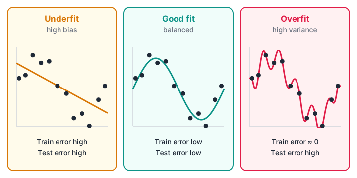
Same data, three models. The underfit line misses the curve, the good fit follows the trend, and the overfit curve chases every noisy point.
Bias and Variance in Plain Words
Two kinds of error explain the three students.
Bias is error from a model's built-in assumptions being too rigid. A straight line has high bias when the truth is curved: no matter how much data you give it, it can never bend. Riya assumed the chapter titles were enough.
Variance is error from a model being too sensitive to which training examples it happened to see. A degree-12 polynomial has high variance: shift one point slightly and the whole curve swings. Aman's answers depended entirely on one specific paper.
Expected error on new data is roughly bias² + variance + irreducible noise. You cannot remove the noise (rain, mood, measurement error). You can only trade bias against variance by choosing the model's complexity.
| High bias (underfit) | Balanced | High variance (overfit) | |
|---|---|---|---|
| Training error | High | Low | Very low |
| Test error | High | Low | High |
| Gap between them | Small | Small | Large |
| Typical cause | Model too simple | Right complexity | Model too complex, too little data |
Train Error vs Test Error as Complexity Grows
The single most useful chart in this topic has model complexity on the x-axis and error on the y-axis.
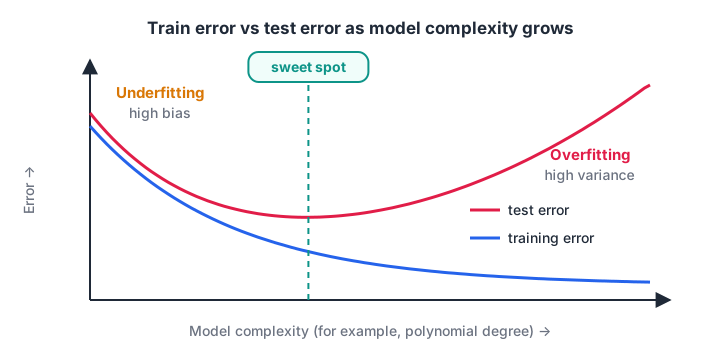
Training error keeps dropping as the model gets more complex. Test error drops, bottoms out at the sweet spot, then rises as variance takes over.
Training error alone is misleading because it always improves as you add complexity. That is why you hold back a test set, or better, use cross-validation. If you have not split data before, the model evaluation metrics guide walks through it.
Quick check
Train MSE is 0.002 and test MSE is 97. What is happening?
A tiny training error with a huge test error means the model memorised training noise, which is high variance.
Lab: Polynomial Fitting in NumPy
Here is the experiment behind both diagrams. The true pattern is a sine wave. You get 15 noisy training points and 100 fresh test points from the same source, then fit polynomials of increasing degree with np.polyfit.
import numpy as np
rng = np.random.default_rng(0)

def true_curve(x):
    return np.sin(2 * np.pi * x)            # the pattern we hope to learn

x_train = np.sort(rng.uniform(0, 1, 15))
y_train = true_curve(x_train) + rng.normal(0, 0.25, 15)
x_test = np.sort(rng.uniform(0, 1, 100))
y_test = true_curve(x_test) + rng.normal(0, 0.25, 100)

print("degree | train MSE | test MSE")
for degree in [1, 2, 3, 5, 9, 12]:
    coefs = np.polyfit(x_train, y_train, degree)
    train_mse = np.mean((np.polyval(coefs, x_train) - y_train) ** 2)
    test_mse = np.mean((np.polyval(coefs, x_test) - y_test) ** 2)
    print(f"{degree:6d} | {train_mse:9.3f} | {test_mse:8.3f}")
Read the output row by row:
- Degrees 1 and 2 have train MSE around 0.19 and test MSE around 0.40. Both are bad: classic underfitting.
- Degree 3 drops both errors sharply (about 0.02 train, 0.08 test). A cubic can bend like one sine cycle, so this is the sweet spot.
- Degree 9 has an even lower training error, yet its test error more than doubles.
- Degree 12 has almost zero training error and a test error near 97. With 13 coefficients and only 15 points, it threads every point and swings wildly between them.
Lower training error at every step, and a much worse model at the end. That is overfitting in one table.
How to Fix Overfitting
1. Get more data
Variance comes from the model reacting to quirks of a small sample. More examples average those quirks out. Keep degree 9 fixed and only change the number of training points:
import numpy as np
rng = np.random.default_rng(0)
f = lambda x: np.sin(2 * np.pi * x)
x_test = np.linspace(0, 1, 200)
y_test = f(x_test) + rng.normal(0, 0.25, 200)

print("points | degree-9 train MSE | degree-9 test MSE")
for n in [15, 50, 200, 1000]:
    x = rng.uniform(0, 1, n)
    y = f(x) + rng.normal(0, 0.25, n)
    c = np.polyfit(x, y, 9)
    tr = np.mean((np.polyval(c, x) - y) ** 2)
    te = np.mean((np.polyval(c, x_test) - y_test) ** 2)
    print(f"{n:6d} | {tr:18.3f} | {te:17.3f}")
With 15 points the test MSE is near 3. With 200 or more, train and test errors meet at about 0.06, which is the noise level itself (0.25² ≈ 0.06). The same flexible model stops overfitting once it has enough evidence.
2. Regularise
Regularisation adds a penalty for large coefficients, so the model prefers smoother curves. Ridge regression uses the penalty alpha × sum of squared coefficients. Keep degree 12 and the original 15 points, and only turn the alpha knob:
import numpy as np
from sklearn.pipeline import make_pipeline
from sklearn.preprocessing import PolynomialFeatures, StandardScaler
from sklearn.linear_model import Ridge

rng = np.random.default_rng(0)
x_train = np.sort(rng.uniform(0, 1, 15)).reshape(-1, 1)
y_train = np.sin(2 * np.pi * x_train).ravel() + rng.normal(0, 0.25, 15)
x_test = np.sort(rng.uniform(0, 1, 100)).reshape(-1, 1)
y_test = np.sin(2 * np.pi * x_test).ravel() + rng.normal(0, 0.25, 100)

print("degree 12 polynomial with ridge regularisation")
print("alpha    | train MSE | test MSE")
for alpha in [1e-10, 1e-4, 1e-2, 1, 100]:
    model = make_pipeline(PolynomialFeatures(12), StandardScaler(), Ridge(alpha=alpha))
    model.fit(x_train, y_train)
    tr = np.mean((model.predict(x_train) - y_train) ** 2)
    te = np.mean((model.predict(x_test) - y_test) ** 2)
    print(f"{alpha:8g} | {tr:9.3f} | {te:8.3f}")
A tiny alpha overfits, a huge alpha underfits, and around alpha = 0.01 the test MSE falls to about 0.07, close to the degree-3 result. Regularisation lets you keep a flexible model and still control variance.
3. Use cross-validation to choose complexity
You should not pick the degree by peeking at the test set, or the test set stops being a fair exam. K-fold cross-validation splits the training data into k parts, trains on k−1, validates on the remaining one, and rotates.
import numpy as np
from sklearn.pipeline import make_pipeline
from sklearn.preprocessing import PolynomialFeatures
from sklearn.linear_model import LinearRegression
from sklearn.model_selection import KFold, cross_val_score

rng = np.random.default_rng(1)
x = rng.uniform(0, 1, 40).reshape(-1, 1)
y = np.sin(2 * np.pi * x).ravel() + rng.normal(0, 0.25, 40)

cv = KFold(n_splits=5, shuffle=True, random_state=0)
results = {}
for degree in range(1, 11):
    model = make_pipeline(PolynomialFeatures(degree), LinearRegression())
    mse = -cross_val_score(model, x, y, cv=cv, scoring="neg_mean_squared_error").mean()
    results[degree] = mse
    print(f"degree {degree:2d}: 5-fold CV MSE = {mse:.3f}")
print("degree chosen by cross-validation:", min(results, key=results.get))
Degrees 3, 4 and 5 score almost the same (about 0.035). The script picks the lowest number, but when scores are this close, a sensible habit is to choose the simplest model, degree 3.
4. Choose a simpler model
Sometimes the cleanest fix is a less flexible model: fewer features, a shallower tree, fewer neurons. In the decision trees lab, limiting max_depth does exactly this.
Quick check
Which fix does NOT reduce overfitting?
Higher degree makes the model more flexible, which increases variance and usually worsens overfitting.
Common Mistakes
- Reporting training accuracy. Recruiters and managers care about performance on unseen data.
- Tuning on the test set. Each peek leaks information. Tune with cross-validation; touch the test set once at the end.
- Thinking more data always helps. More data fixes variance, not bias. A straight line stays a straight line with a million points.
- Forgetting to scale before regularising. Ridge penalises coefficient size, so features on very different scales get penalised unfairly. Put
StandardScalerin the pipeline.
Learning to diagnose these problems on messy real datasets is easier with someone checking your reasoning. Structured machine learning training in Indore at Debugshala includes this kind of model-tuning practice.
Key takeaways
- Underfitting is high bias: errors are high on both training and test data.
- Overfitting is high variance: training error is low, test error is much higher.
- Training error always falls as complexity grows; test error is U-shaped.
- More data, regularisation, cross-validation and simpler models all reduce overfitting.
- Pick complexity with cross-validation and keep the test set for the final check.
FAQ
How do I know if my model is overfitting?
Compare training and validation (or test) scores. A large gap, such as 99% training accuracy with 75% validation accuracy, signals overfitting. Learning curves that plot both errors against training size make the gap easy to see.
Is some overfitting acceptable?
A small gap between training and test performance is normal and expected. What matters is the test or cross-validation score. If a slightly more complex model has a slightly bigger gap but a better test score, it is usually the better choice.
What is the difference between L1 and L2 regularisation?
L2 (ridge) shrinks all coefficients smoothly towards zero. L1 (lasso) can push some coefficients exactly to zero, which also performs feature selection. scikit-learn provides both as Ridge and Lasso, documented at scikit-learn.org.
Where can I practise bias-variance problems with a trainer in Indore?
Debugshala, at C.S. Naidu Arcade in Old Palasia, Indore, runs a Machine Learning course with offline classes taught in English and Hindi. It is open to fresh graduates, non-IT learners and people with a year gap, and you can try a free demo class first. For quick self-tests, use the MCQs on Debugshala Test.
From the team behind this site
Go further with the Data Science & AI Course at Debugshala
These tutorials are written by Debugshala, a training and placement institute at Old Palasia, Indore. The classroom course adds live mentoring, real projects and interview preparation.
- Offline classes at Old Palasia, Indore
- Free demo class before you pay
- Non-IT, fresher and year-gap friendly
- Placement assistance
700+ students placed · 200+ hiring partners · 4.9★ Google rating
