

Model Evaluation Metrics: Accuracy, F1, ROC-AUC, RMSE and More
Model evaluation metrics with runnable sklearn code: train/test split, confusion matrix, precision, recall, F1, ROC-AUC, MAE, RMSE, R² and when to use each.
Suppose you are the security guard at a mall entrance in Vijay Nagar, and your manager says you will be graded on "accuracy". Out of 1,000 visitors a day, maybe 2 are shoplifters. You realise you can wave everyone through and be right 998 times. Accuracy 99.8%. Zero thieves caught.
Your manager changes the rules. Now you are graded on how many of the actual shoplifters you stop. You start checking every bag. You catch both thieves, but 300 annoyed shoppers complain.
Neither grading scheme is wrong. Each one rewards a different behaviour. Picking how to score a model is the same decision, and it shapes the model you end up with.
Train/Test Split: Grading on Unseen Questions
Map the mall to ML. The visitors your model learns from are the training set. The visitors it is judged on must be different ones, the test set. Otherwise you are grading a student on the exact questions they memorised, the trap explained in the overfitting and bias-variance lab.
Model evaluation is the practice of measuring a trained model's performance on held-out data using metrics that reflect the real cost of its mistakes.
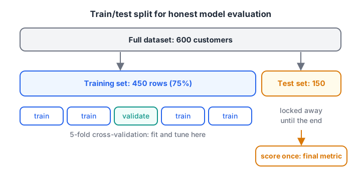
Split once at the start. Fit and tune only on the training part (cross-validation lives inside it). Score on the test part once, at the end.
Three habits make the split trustworthy:
- Use
stratify=yfor classification so the rare class appears in both parts in the same proportion. - Fix
random_stateso you and your teammates get the same split. - For time-based data (sales, stock, footfall), split by date instead of randomly: train on the past, test on the future.
Accuracy vs Precision, Recall and F1
Every prediction of a yes/no classifier lands in one of four boxes, called the confusion matrix.
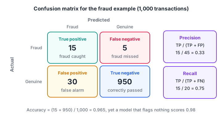
Rows are what really happened, columns are what the model predicted. Precision reads down the "predicted positive" column; recall reads across the "actually positive" row.
From those four counts you get the main classification metrics:
| Metric | Formula | Question it answers |
|---|---|---|
| Accuracy | (TP + TN) / all | How often is the model right overall? |
| Precision | TP / (TP + FP) | When it says "yes", how often is it right? |
| Recall | TP / (TP + FN) | Of all real "yes" cases, how many did it catch? |
| F1 | 2·P·R / (P + R) | A single balance of precision and recall |
Why accuracy misleads on imbalanced data
Here is the guard's problem with card fraud: 20 frauds hidden in 1,000 transactions. Compare a lazy model that always says "genuine" with a real one.
# 1,000 card transactions: 20 are fraud (1), 980 are genuine (0)
y_true = [1] * 20 + [0] * 980

lazy = [0] * 1000                                  # always says "genuine"
print("Lazy model accuracy:", sum(t == p for t, p in zip(y_true, lazy)) / 1000)

# A real model: catches 15 frauds, misses 5, wrongly flags 30 genuine ones
model = [1] * 15 + [0] * 5 + [1] * 30 + [0] * 950
tp = sum(t == 1 and p == 1 for t, p in zip(y_true, model))
fn = sum(t == 1 and p == 0 for t, p in zip(y_true, model))
fp = sum(t == 0 and p == 1 for t, p in zip(y_true, model))
tn = sum(t == 0 and p == 0 for t, p in zip(y_true, model))
precision, recall = tp / (tp + fp), tp / (tp + fn)
f1 = 2 * precision * recall / (precision + recall)
print(f"TP={tp} FN={fn} FP={fp} TN={tn}")
print(f"accuracy={(tp + tn) / 1000:.3f} precision={precision:.3f} recall={recall:.3f} f1={f1:.3f}")
The lazy model scores 98% accuracy. The useful model scores only 96.5%, yet it catches 75% of frauds (recall 0.75). Its precision of 0.33 means one in three flags is real fraud, which may be perfectly acceptable if a quick SMS check clears the rest. Accuracy picked the wrong winner.
Quick check
A model flags 50 transactions as fraud and 40 of them really are fraud. What is its precision?
Precision = TP / (TP + FP) = 40 / 50 = 0.8.
Lab: Evaluating a Churn Model with scikit-learn
Now a full workflow. You will generate 600 inline customer records for a broadband provider (tenure in months and recent complaints), predict who churns, and print every metric in one go.
import numpy as np
from sklearn.model_selection import train_test_split
from sklearn.linear_model import LogisticRegression
from sklearn.metrics import confusion_matrix, classification_report, roc_auc_score

rng = np.random.default_rng(7)
n = 600
tenure = rng.integers(1, 60, n)                # months as a customer
complaints = rng.poisson(1.0, n)               # complaints last quarter
score = -0.08 * tenure + 0.9 * complaints + rng.normal(0, 1, n)
churn = (score > 0).astype(int)                # 1 = customer left
X = np.column_stack([tenure, complaints])

X_tr, X_te, y_tr, y_te = train_test_split(X, churn, test_size=0.25, stratify=churn, random_state=0)
clf = LogisticRegression().fit(X_tr, y_tr)
pred = clf.predict(X_te)
proba = clf.predict_proba(X_te)[:, 1]

print("train rows:", len(X_tr), "test rows:", len(X_te), "churn rate:", round(churn.mean(), 2))
print("confusion matrix [[TN FP] [FN TP]]:\n", confusion_matrix(y_te, pred))
print(classification_report(y_te, pred, digits=3))
print("ROC-AUC:", round(roc_auc_score(y_te, proba), 3))
On the 150 test customers you should see accuracy of 0.88, but for the churn class (label 1) a recall of about 0.65: the model misses 11 of 31 leavers. If the retention team can call 40 people a week, that recall is the number to push up.
The ROC-AUC idea
A classifier really outputs a probability, and predict simply cuts it at 0.5. Move that threshold and you trade precision for recall:
import numpy as np
from sklearn.model_selection import train_test_split
from sklearn.linear_model import LogisticRegression
from sklearn.metrics import precision_score, recall_score

rng = np.random.default_rng(7)
tenure = rng.integers(1, 60, 600)
complaints = rng.poisson(1.0, 600)
churn = ((-0.08 * tenure + 0.9 * complaints + rng.normal(0, 1, 600)) > 0).astype(int)
X = np.column_stack([tenure, complaints])
X_tr, X_te, y_tr, y_te = train_test_split(X, churn, test_size=0.25, stratify=churn, random_state=0)
proba = LogisticRegression().fit(X_tr, y_tr).predict_proba(X_te)[:, 1]

print("threshold | precision | recall | flagged")
for t in [0.2, 0.35, 0.5, 0.65, 0.8]:
    pred = (proba >= t).astype(int)
    p = precision_score(y_te, pred, zero_division=0)
    r = recall_score(y_te, pred)
    print(f"{t:9.2f} | {p:9.3f} | {r:6.3f} | {pred.sum():7d}")
At threshold 0.35 the model flags 42 customers and catches about 87% of leavers, which fits a team that can make 40-odd calls. At 0.8 every flag is correct, but it catches only a quarter of them.
The ROC curve plots the true positive rate (recall) against the false positive rate for every possible threshold. AUC, the area under that curve, condenses it into one number: the probability that a randomly chosen churner gets a higher score than a randomly chosen loyal customer.
0.5 is coin-flipping, 1.0 is perfect ranking. Our 0.918 says the model ranks well, even if the default threshold is not ideal for the business.
Regression Metrics: MAE, RMSE and R²
When the target is a number, like monthly rent, you measure how far predictions land from the truth.
- MAE (mean absolute error): the average size of a miss, in the target's own units. Easy to explain.
- RMSE (root mean squared error): squares errors before averaging, so one big miss hurts a lot. Also in the target's units.
- R² (coefficient of determination): the share of the target's variation the model explains. 1 is perfect, 0 is no better than always predicting the average, and it can go negative.
import numpy as np
from sklearn.metrics import mean_absolute_error, mean_squared_error, r2_score

# Monthly rent (rupees) for 8 flats: actual vs a model's prediction
actual    = np.array([12000, 15000, 9000, 22000, 18000, 11000, 30000, 14000])
predicted = np.array([13000, 14000, 9500, 20000, 18500, 12500, 24000, 14500])

mae = mean_absolute_error(actual, predicted)
rmse = np.sqrt(mean_squared_error(actual, predicted))
r2 = r2_score(actual, predicted)
print(f"MAE  = Rs {mae:,.0f}  (average miss)")
print(f"RMSE = Rs {rmse:,.0f}  (punishes big misses more)")
print(f"R2   = {r2:.3f}  (share of rent variation explained)")
print("errors:", (predicted - actual).tolist())
MAE is Rs 1,625 but RMSE is Rs 2,372. The gap comes almost entirely from one flat where the model under-predicted by Rs 6,000. When RMSE is much bigger than MAE, look for a few large misses.
Quick check
MAE is 1,600 and RMSE is 4,800 on the same predictions. What does that suggest?
RMSE squares errors, so it grows much faster than MAE when a few misses are large.
Choosing a Metric for the Business Problem
Before you train anything, ask: which mistake costs more, and who pays for it?
| Business problem | Costly mistake | Lead metric |
|---|---|---|
| Cancer or disease screening | Missing a sick patient (FN) | Recall |
| Spam filter for work email | Hiding a real email (FP) | Precision |
| Loan default prediction | Both, unequally | F1 or cost-weighted score, plus ROC-AUC for ranking |
| Retention calls with a fixed team | Wasted calls and missed churners | Precision and recall at the team's capacity |
| Delivery time estimate | Occasional huge delays upset customers | RMSE |
| Rent or price estimate shown to users | Typical error matters | MAE |
| Balanced classes, equal costs | Any error | Accuracy is fine |
Then report the metric with a baseline: "With 42 calls we reach 87% of the customers who would leave; 42 random calls would reach about 28%." That sentence lands far better with a manager than "F1 = 0.69".
Quick check
For screening a serious disease, which metric should you prioritise?
Missing a sick patient (a false negative) is the costly error, so you want high recall.
Common Mistakes
- Scoring on training data. Always use a held-out test set or cross-validation.
- Reporting accuracy on imbalanced classes. Report precision and recall for the rare class.
- Using the default 0.5 threshold blindly. Pick the threshold that fits the business capacity and cost.
- Comparing RMSE across different targets. RMSE is in target units, so Rs 2,000 and 2 minutes are not comparable. Use R² or a percentage error for cross-problem comparison.
- Leaking the future. Shuffling time-series data before splitting lets the model peek at tomorrow.
If you want a trainer to review your evaluation choices on real projects, Debugshala's hands-on ML classes in Indore cover metrics alongside model building. The decision trees lab is a good model to practise these metrics on.
Key takeaways
- Split data first; fit on training data and score once on the test set.
- Accuracy can reward a useless model when classes are imbalanced.
- Precision asks "are my flags right?"; recall asks "did I catch them all?"; F1 balances the two.
- ROC-AUC measures ranking quality across all thresholds; choose the actual threshold from business capacity.
- MAE, RMSE and R² describe regression errors; a big RMSE-to-MAE gap means a few large misses.
FAQ
What is a good accuracy for a machine learning model?
It depends on the baseline. If 98% of cases belong to one class, 98% accuracy is what a model that predicts nothing achieves. Compare your model with a simple baseline and with the metric that reflects business cost.
What is the difference between precision and recall?
Precision is the share of predicted positives that are truly positive. Recall is the share of actual positives the model found. Raising the threshold usually increases precision and lowers recall.
When should I use ROC-AUC instead of F1?
Use ROC-AUC to compare how well models rank cases, independent of any threshold. Use F1 (or precision and recall) once you have chosen a threshold and care about the actual decisions. The scikit-learn model evaluation guide lists all the options.
Does Debugshala teach model evaluation in its Indore classes?
Debugshala's Machine Learning course is taught offline at the Old Palasia campus in Indore, in English and Hindi, and accepts fresh graduates and learners from non-IT backgrounds. You can attend a free demo class before paying to see how the sessions run. To test yourself on concepts like these, try the MCQs on Debugshala Test.
From the team behind this site
Go further with the Data Science & AI Course at Debugshala
These tutorials are written by Debugshala, a training and placement institute at Old Palasia, Indore. The classroom course adds live mentoring, real projects and interview preparation.
- Offline classes at Old Palasia, Indore
- Free demo class before you pay
- Non-IT, fresher and year-gap friendly
- Placement assistance
700+ students placed · 200+ hiring partners · 4.9★ Google rating
