

Support Vector Machines (SVM) Explained: Margins and Kernels
Support vector machines explained: maximum margin, support vectors, the C parameter, the kernel trick, RBF gamma and when SVMs beat other models, in Python.
The Indore Municipal Corporation wants to lay a new road between two colonies. Houses from Colony A sit on one side and houses from Colony B on the other. Many straight roads would keep the colonies apart, but the planners want the widest road possible, so nobody's gate opens straight onto traffic.
Notice what decides the road. Houses deep inside each colony don't matter. Only the few edge houses that the kerbs would touch fix its position and width.
What is a support vector machine?
Map the road project to machine learning:
- Each house is a training row and its colony is the class label.
- The centre line of the road is the decision boundary, a line in 2D or a hyperplane in more dimensions.
- The road's width is the margin.
- The edge houses that touch the kerbs are the support vectors.
A support vector machine (SVM) is a supervised learning algorithm that classifies data by finding the hyperplane that separates the classes with the maximum margin, where the margin is set only by the training points closest to the boundary, called support vectors.
This tutorial covers classification with scikit-learn 1.7's SVC; the same idea powers SVR for regression. It follows Naive Bayes, which reasons with probabilities; an SVM reasons purely with geometry.
How does an SVM find the maximum margin?
A linear SVM scores every point with f(x) = w · x + b. The sign of f(x) gives the class, and the boundary is where f(x) = 0. The SVM picks w and b so that the support vectors land exactly on f(x) = +1 and f(x) = −1, and every other point lies beyond them.
The distance between those two kerb lines is 2 / ||w||. A wider margin means a smaller w, so training an SVM is an optimisation problem: make ||w|| as small as possible while keeping every point on its correct side.
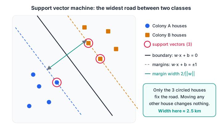
The solid line is the decision boundary. The three circled houses are the support vectors; every other house could move without changing the road.
Here is that picture in code, with ten houses:
import numpy as np
from sklearn.svm import SVC

# houses: (km east, km north). 0 = Colony A, 1 = Colony B
X = np.array([[1.0, 1.0], [1.5, 2.0], [2.0, 1.2], [1.2, 2.6], [2.4, 2.2],
              [4.0, 4.2], [4.6, 3.4], [5.0, 4.8], [3.8, 5.0], [5.4, 3.9]])
y = np.array([0, 0, 0, 0, 0, 1, 1, 1, 1, 1])

svm = SVC(kernel="linear", C=1000).fit(X, y)       # huge C = (almost) hard margin
w, b = svm.coef_[0], svm.intercept_[0]
print("weights w:", w.round(3), " bias b:", round(b, 3))
print("road width (margin) = 2/||w|| =", round(2 / np.linalg.norm(w), 3), "km")
print("support vectors:", svm.support_vectors_.tolist())
print("decision_function on support vectors:", svm.decision_function(svm.support_vectors_).round(2))
print("new house at (3, 3) ->", "Colony", "AB"[svm.predict([[3, 3]])[0]])
The SVM finds a road about 2.5 km wide, and only three of the ten houses are support vectors. Their decision values are exactly −1 and +1, as the theory says. A new house at (3, 3) scores just below zero, so it falls on Colony A's side.
The widest road matters because a boundary hugging one colony would misclassify the first slightly out-of-place new house.
Quick check
Which training points determine the position of an SVM's decision boundary?
Only the support vectors on or inside the margin affect the solution. Points far away can move without changing it.
What does the C parameter do in SVM?
Real data is rarely so tidy, and often no straight road separates everything. The soft-margin SVM allows some points inside the margin or on the wrong side, and charges a penalty for each one.
C sets the price of those violations:
- Small C makes violations cheap. The SVM chooses a wide, relaxed margin and accepts some training mistakes. Many points end up as support vectors. This leans towards underfitting.
- Large C makes violations expensive. The SVM bends over backwards to classify every training point, with a narrow margin. This leans towards overfitting.
from sklearn.datasets import make_moons
from sklearn.model_selection import cross_validate
from sklearn.pipeline import make_pipeline
from sklearn.preprocessing import StandardScaler
from sklearn.svm import SVC

X, y = make_moons(n_samples=300, noise=0.35, random_state=2)

print("      C | support vectors | train acc | CV acc")
for C in [0.01, 0.1, 1, 10, 100, 1000]:
    model = make_pipeline(StandardScaler(), SVC(kernel="rbf", gamma=2, C=C))
    res = cross_validate(model, X, y, cv=5, return_train_score=True)
    n_sv = model.fit(X, y)[-1].n_support_.sum()
    print(f"{C:7} | {n_sv:15d} | {res['train_score'].mean():9.3f} | {res['test_score'].mean():.3f}")
As C grows from 0.01 to 1,000, training accuracy climbs from about 0.87 to about 0.93 and the number of support vectors falls from all 300 rows to about 100. Cross-validated accuracy peaks around C = 1 and then drops to about 0.80: a larger C is chasing noise. This is the bias-variance trade-off again, with C as the dial.
What is the kernel trick in SVM?
Some classes can't be separated by any straight line. Picture a chai stall's daily sales: normal days sell 30 to 70 cups, while unusual days (a bandh, or a festival rush) sell very few or very many. On a number line the "normal" class sits in the middle, flanked by "unusual" on both sides. One cut can't split that.
The fix is to add a dimension. Give every point a second coordinate, x², and the middle values sit low while the extremes rise high. Now a flat line separates them.
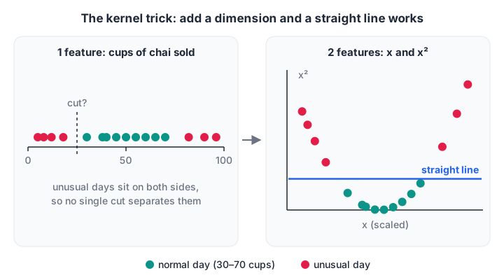
Left: no single threshold splits normal days from unusual ones. Right: after adding x², a straight line does the job.
import numpy as np
from sklearn.svm import SVC

# 1-D feature: daily chai cups sold. Class 1 = a "normal" day (middle), 0 = unusual (very low or very high)
x = np.array([5, 12, 18, 40, 45, 50, 55, 60, 82, 90, 96, 30, 70, 8, 65, 38])
y = np.array([0, 0, 0, 1, 1, 1, 1, 1, 0, 0, 0, 1, 1, 0, 1, 1])
x_s = (x - x.mean()) / x.std()

flat = SVC(kernel="linear", C=10).fit(x_s.reshape(-1, 1), y)
lifted = np.column_stack([x_s, x_s ** 2])            # add a new dimension: x squared
curved = SVC(kernel="linear", C=10).fit(lifted, y)
print("linear SVM on x alone      :", flat.score(x_s.reshape(-1, 1), y))
print("linear SVM on (x, x squared):", curved.score(lifted, y))
rbf = SVC(kernel="rbf", C=10).fit(x_s.reshape(-1, 1), y)
print("RBF kernel on x alone      :", rbf.score(x_s.reshape(-1, 1), y))
A linear SVM on raw sales gets 0.75 of the days right; with x² added it gets all of them. The RBF kernel does the same with no manual feature.
That last line is the kernel trick. An SVM's maths only ever needs the similarity between pairs of points, never the new coordinates themselves.
A kernel is a function that computes that similarity as if the points had been mapped into a higher-dimensional space, without building the space. The RBF kernel corresponds to an infinite-dimensional space, yet costs one exponential per pair.
Common SVM kernels
| Kernel | Similarity it measures | Key parameters | Use it when |
|---|---|---|---|
linear |
Plain dot product | C | Many features (text), or a straight boundary is enough |
poly |
Polynomial of the dot product | C, degree, coef0 | Interactions of a known order matter |
rbf (default) |
Closeness, decaying with distance | C, gamma | Good general default for curved boundaries |
sigmoid |
tanh of the dot product | C, gamma, coef0 | Rarely; mostly of historical interest |
Gamma in the RBF kernel
gamma controls how far one training point's influence reaches. Small gamma gives each point a wide reach, so the boundary is smooth. Large gamma shrinks the reach to a tiny bubble around each point, so the boundary wraps around individual rows.
from sklearn.datasets import make_circles, make_moons
from sklearn.model_selection import cross_validate
from sklearn.pipeline import make_pipeline
from sklearn.preprocessing import StandardScaler
from sklearn.svm import SVC

X, y = make_circles(n_samples=400, factor=0.4, noise=0.12, random_state=0)
for kernel in ["linear", "poly", "rbf"]:
    model = make_pipeline(StandardScaler(), SVC(kernel=kernel, degree=2))
    acc = cross_validate(model, X, y, cv=5)["test_score"].mean()
    print(f"circles, {kernel:>6} kernel: CV accuracy {acc:.3f}")

X, y = make_moons(n_samples=300, noise=0.35, random_state=2)
print("\nmoons:  gamma | train acc | CV acc")
for gamma in [0.01, 0.1, 1, 10, 100]:
    model = make_pipeline(StandardScaler(), SVC(kernel="rbf", C=1, gamma=gamma))
    res = cross_validate(model, X, y, cv=5, return_train_score=True)
    print(f"{gamma:13} | {res['train_score'].mean():9.3f} | {res['test_score'].mean():.3f}")
On the circles data, a linear kernel scores about 0.54, barely above guessing, while the polynomial and RBF kernels score close to 1.0.
On the noisier moons, gamma = 100 reaches about 0.98 on training rows but only 0.75 in cross-validation, a clear sign of overfitting. Tune C and gamma together with a grid on a log scale, as shown in hyperparameter tuning.
Quick check
An RBF SVM scores 99% on training data and 74% in cross-validation. Which change is most likely to help?
High training and low validation accuracy means overfitting. Smaller gamma and smaller C both smooth the boundary.
SVM in practice: scaling, probabilities and speed
Always scale features
An SVM measures distances, so a rupee column swamps a years column, as in KNN. Keep StandardScaler in the pipeline.
Probabilities are optional and slower
SVC outputs a decision score, not a probability. SVC(probability=True) adds probabilities by fitting an extra calibration model with internal cross-validation, which makes training several times slower. If you only need a ranking, use decision_function.
Speed limits
Kernel SVM training time grows roughly between the square and the cube of the number of rows. It's comfortable at a few thousand rows and painful at a few hundred thousand. For large data, LinearSVC or SGDClassifier(loss="hinge") train a linear SVM much faster, and tree ensembles such as random forests are often a better choice.
| Strengths | Weaknesses |
|---|---|
| Strong accuracy on small and medium data | Slow on large datasets |
| Works well with many features, even more features than rows | Needs feature scaling |
| Kernels give flexible boundaries | C and gamma must be tuned together |
| Only support vectors are needed at prediction time | No native probabilities |
| Max-margin idea resists overfitting | Hard to explain to non-technical users |
Common SVM mistakes
- Skipping the scaler. Unscaled features distort every distance and kernel value.
- Tuning C and gamma separately. They interact; search them together.
- Using the RBF kernel on large text data. A linear kernel is usually as accurate and far faster there.
- Turning on probability=True by habit. It slows training and is only needed when you truly need probabilities.
- Reading coef_ from a kernel SVM. Only the linear kernel has feature weights you can interpret.
The maths behind SVMs is easier to absorb with a trainer at a whiteboard, which is how hands-on ML training at Debugshala's Indore campus teaches it. When you're ready, attempt SVM and kernel questions on Debugshala Test. The series continues with decision trees.
Key takeaways
- An SVM separates classes with the widest possible margin; only the support vectors set it.
- C trades margin width against training mistakes: small C is relaxed, large C is strict.
- Kernels let SVMs draw curved boundaries by measuring similarity in a richer space, without building that space.
- RBF is the default kernel; tune C and gamma together and always scale features.
- SVMs shine on small and medium datasets and slow down sharply as rows grow.
FAQ
What is a support vector in SVM?
A support vector is a training point that lies on the edge of the margin, or inside it, closest to the decision boundary. These points alone determine where the boundary goes. In a well-separated dataset they are often only a handful of rows, which is why SVMs can store a compact model.
What is the difference between SVM and logistic regression?
Both draw a linear boundary, but they choose it differently. Logistic regression fits probabilities using every point, while a linear SVM maximises the margin using only the support vectors. With kernels, SVMs also handle curved boundaries directly. Logistic regression gives calibrated probabilities more naturally and scales better to large datasets.
Which kernel should I use in SVM?
Start with the RBF kernel for most tabular problems, since it handles curved boundaries and has only two parameters. Use the linear kernel when you have many features, such as text, or when you need interpretable weights. Choose between them with cross-validation rather than guesswork.
Is SVM still used in industry?
Yes, though less than before. SVMs remain common for text classification, small datasets with many features, and problems such as image or signal classification where carefully built features exist. For large tabular datasets, gradient boosting usually wins, and deep learning dominates raw images and audio.
Where can I learn SVM and other ML algorithms in Indore?
Debugshala teaches SVMs alongside the other supervised learning algorithms in its Machine Learning course at Old Palasia, Indore. Classes run offline in English and Hindi, and freshers, non-IT graduates and people with a year gap can join. For admissions, call +91-8982385539 or email info@debugshala.com.
From the team behind this site
Go further with the Data Science & AI Course at Debugshala
These tutorials are written by Debugshala, a training and placement institute at Old Palasia, Indore. The classroom course adds live mentoring, real projects and interview preparation.
- Offline classes at Old Palasia, Indore
- Free demo class before you pay
- Non-IT, fresher and year-gap friendly
- Placement assistance
700+ students placed · 200+ hiring partners · 4.9★ Google rating
