

Anomaly Detection in Machine Learning: Isolation Forest, LOF
Anomaly detection techniques in Python: Isolation Forest, Local Outlier Factor, One-Class SVM, novelty detection, thresholds and how to evaluate detectors.
Think of Meena, who has handled the same customers at a small bank branch in Vijay Nagar for ten years. She knows that Mr Joshi withdraws about ₹5,000 every Saturday morning and that the college student in the next lane pays small UPI amounts at tea stalls all day.
One Tuesday at 3:10 a.m., Mr Joshi's card buys ₹48,000 of electronics in a city he has never visited. Nobody told Meena a rule like "flag purchases over ₹40,000 at night". She simply knows his normal, and this is not it.
Teaching a computer to have Meena's sense of "this is not normal" is what anomaly detection is about.
What is anomaly detection in machine learning?
Map the bank to the data:
- Each transaction is a row, with features such as amount, hour and distance from home.
- Meena's memory of each customer's habits is the model of normal behaviour.
- The 3 a.m. purchase is an anomaly, and her feeling of surprise is an anomaly score.
- Deciding when surprise is strong enough to call the customer is the threshold.
Anomaly detection is the process of learning what normal data looks like and flagging observations that deviate from it strongly enough to be suspicious, typically when anomalies are rare and few labelled examples exist.
The single-column rules (z-score, IQR, MAD) live in outlier detection. This tutorial covers machine learning techniques that look at many features together and catch points that seem normal on every column but strange in combination. Code targets scikit-learn 1.7.
Three kinds of anomalies
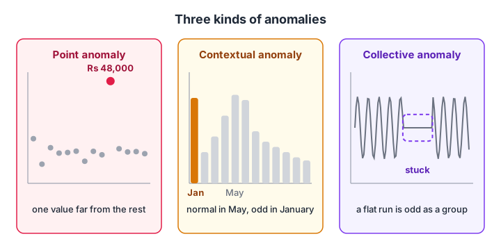
A point anomaly is odd on its own, a contextual anomaly is odd for its time or place, and a collective anomaly is a run of values that is odd only as a group.
- Point: a ₹48,000 purchase on a card that averages ₹1,200.
- Contextual: 400 ice creams sold is ordinary in May, suspicious in January.
- Collective: a heart monitor stuck on one healthy value for 20 seconds is broken.
Most tabular techniques below target point anomalies. Contextual ones need the context as a feature (month, hour, store), and collective ones need time-window features, as built in time series analysis.
Supervised, semi-supervised or unsupervised?
How you frame the problem depends on the labels you have.
| Setting | Labels you have | Typical method | Example |
|---|---|---|---|
| Supervised | Many confirmed anomalies and normals | Classifier with class weights | Years of tagged insurance fraud |
| Semi-supervised (novelty detection) | A clean set of normal data only | One-Class SVM, LOF with novelty=True |
Vibration readings from a healthy new motor |
| Unsupervised (outlier detection) | No labels; data contains some anomalies | Isolation Forest, LOF | Last month's raw transactions |
If you do have plenty of labelled fraud, treat it as a classification problem with a rare class and use the tools from handling imbalanced data. Anomaly detection shines when labels are scarce, late or missing, which is most of the time.
How does Isolation Forest detect anomalies?
Isolation Forest flips the question. Instead of describing normal points, it asks how quickly random cuts can separate a point from all the others.
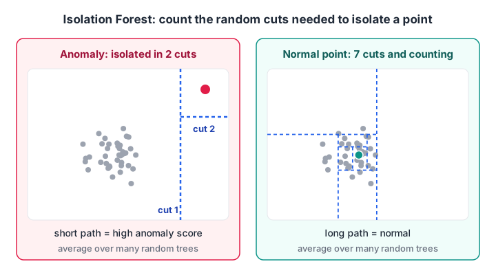
Random splits isolate a lonely point in very few steps. The shorter the average path across many random trees, the more anomalous the point.
The algorithm works like this:
- Pick a random feature and a random cut value between its minimum and maximum.
- Split the data and repeat inside each part until every point stands alone.
- Record how many splits each point needed (its path length).
- Repeat with many random trees and average the path lengths.
- Short average paths mean anomalies; long ones mean normal points buried in a crowd.
It is fast, needs no scaling and, like a random forest, gains strength from averaging many random trees.
import numpy as np
from sklearn.ensemble import IsolationForest

rng = np.random.default_rng(0)
# 1000 normal card transactions: amount (Rs), hour of day, km from home
normal = np.column_stack([rng.gamma(2, 600, 1000),
                          rng.normal(14, 3, 1000).clip(6, 23),
                          rng.exponential(4, 1000)])
# 15 frauds: large amounts, late night, far from home
fraud = np.column_stack([rng.uniform(15000, 60000, 15),
                         rng.uniform(0, 4, 15),
                         rng.uniform(300, 1500, 15)])
X = np.vstack([normal, fraud])
y = np.r_[np.zeros(1000), np.ones(15)]          # used only to check the result

iso = IsolationForest(n_estimators=200, contamination=0.015, random_state=0)
pred = iso.fit_predict(X)                       # -1 = anomaly, 1 = normal
flagged = pred == -1
print("flagged:", flagged.sum(), "| true frauds among them:", int(y[flagged].sum()))

score = -iso.score_samples(X)                   # higher = more anomalous
top = np.argsort(score)[::-1][:5]
print("top 5 rows:", top, "labels:", y[top])
Sixteen rows are flagged: all 15 planted frauds plus one false alarm. contamination is your guess at the anomaly share, and scikit-learn uses it only to set the score cut-off.
Quick check
Why does Isolation Forest give anomalies short path lengths?
Random cuts quickly carve out a lonely point, while a point inside a dense cluster needs many cuts.
Quick check
Your fraud model shows 99.2% accuracy on data with 0.8% fraud. What should you check first?
Predicting "not fraud" for every row already gives 99.2% accuracy. Precision, recall and average precision reveal the truth.
Local Outlier Factor for uneven density
Sometimes a point is odd only relative to its own neighbourhood. Picture dense kirana stores in one market and scattered godowns on the bypass. A shop just outside the tight kirana cluster is odd, though it sits closer to the centre than any godown.
Local Outlier Factor (LOF) compares each point's local density with the density around its nearest neighbours. A score near 1 means "as dense as my neighbours"; well above 1 means "much lonelier than my neighbours".
import numpy as np
from sklearn.neighbors import LocalOutlierFactor

rng = np.random.default_rng(1)
dense = rng.normal([0, 0], 0.3, (200, 2))       # tight cluster
sparse = rng.normal([8, 8], 2.0, (100, 2))      # loose cluster
odd = np.array([[1.6, 1.6]])                    # just outside the tight cluster
X = np.vstack([dense, sparse, odd])

centre_dist = np.linalg.norm(X - X.mean(axis=0), axis=1)
print("rank of the odd point by global distance:",
      int((centre_dist > centre_dist[-1]).sum()) + 1, "of", len(X))

lof = LocalOutlierFactor(n_neighbors=20)
lof.fit_predict(X)
lof_score = -lof.negative_outlier_factor_
print("rank of the odd point by LOF score:",
      int((lof_score > lof_score[-1]).sum()) + 1, "of", len(X))
print(f"LOF score of odd point: {lof_score[-1]:.1f}, median score: {np.median(lof_score):.2f}")
A global distance check ranks the odd point dead last, 301 of 301, because it sits near the overall centre. LOF ranks it first. LOF uses distances, so scale your features first, just as with k-nearest neighbours. For a related density idea used in clustering, see DBSCAN, which labels low-density points as noise.
Comparing anomaly detection techniques
No single detector wins everywhere. When you have even a small labelled sample, compare a few on it. Accuracy is useless here, because predicting "normal" for everything already scores 99%. Use average precision (area under the precision-recall curve) and precision at k, the share of real anomalies in the top k alerts.
import numpy as np
from sklearn.datasets import make_blobs
from sklearn.preprocessing import StandardScaler
from sklearn.ensemble import IsolationForest
from sklearn.neighbors import LocalOutlierFactor
from sklearn.svm import OneClassSVM
from sklearn.covariance import EllipticEnvelope
from sklearn.metrics import average_precision_score

rng = np.random.default_rng(2)
inliers, _ = make_blobs(n_samples=950, centers=3, n_features=4, random_state=2)
outliers = rng.uniform(-15, 15, (50, 4))
X = StandardScaler().fit_transform(np.vstack([inliers, outliers]))
y = np.r_[np.zeros(950), np.ones(50)]

detectors = {
    "IsolationForest": lambda: -IsolationForest(random_state=0).fit(X).score_samples(X),
    "LOF": lambda: -LocalOutlierFactor(n_neighbors=30).fit(X).negative_outlier_factor_,
    "OneClassSVM": lambda: -OneClassSVM(nu=0.05, gamma="scale").fit(X).score_samples(X),
    "EllipticEnvelope": lambda: -EllipticEnvelope(random_state=0).fit(X).score_samples(X),
}
for name, get_score in detectors.items():
    s = get_score()
    p_at_50 = y[np.argsort(s)[::-1][:50]].mean()
    print(f"{name:>16}: average precision {average_precision_score(y, s):.2f}, precision@50 {p_at_50:.2f}")
Normal data here forms three clusters. Isolation Forest and LOF catch all 50 anomalies. Elliptic Envelope assumes one oval cloud and trails, as does One-Class SVM, which is sensitive to its settings.
| Technique | Core idea | Strengths | Weaknesses |
|---|---|---|---|
| Isolation Forest | Anomalies need few random splits | Fast, scales to many rows and features, no scaling needed | Weaker on purely local anomalies |
| Local Outlier Factor | Lower density than neighbours | Finds local anomalies in uneven data | Slow on very large data; needs scaling |
| One-Class SVM | Boundary around normal data | Flexible shapes with the RBF kernel | Sensitive to nu and gamma; slow beyond ~50k rows |
| Elliptic Envelope | Distance from one Gaussian cloud | Simple, good for one roughly normal cluster | Fails with several clusters or skewed data |
| PCA or autoencoder reconstruction | Anomalies rebuild poorly | Works on images, sensors, many correlated features | Needs clean training data and a threshold |
The last row reuses the reconstruction error idea from PCA and dimensionality reduction; autoencoders are its neural version. The One-Class SVM borrows the kernel trick from support vector machines.
Novelty detection: training on clean data
With a clean sample of normal behaviour, fit on it and score new rows as they arrive. The classic case: record a healthy machine for a week, then watch for anything unlike that week.
import numpy as np
from sklearn.neighbors import LocalOutlierFactor

rng = np.random.default_rng(3)
# one week of a healthy pump: temperature (C) and vibration (mm/s)
healthy = np.column_stack([rng.normal(55, 2, 2000), rng.normal(2.0, 0.3, 2000)])

model = LocalOutlierFactor(n_neighbors=25, novelty=True).fit(healthy)

new_readings = np.array([[56.0, 2.1],    # normal
                         [54.2, 1.8],    # normal
                         [57.0, 4.5],    # vibration spike: bearing wear?
                         [68.0, 2.2]])   # overheating
print("prediction (1 normal, -1 anomaly):", model.predict(new_readings))
print("anomaly scores:", np.round(-model.score_samples(new_readings), 2))
With novelty=True, LOF offers predict and score_samples for unseen data. Do not call fit_predict in this mode.
How do you choose the anomaly threshold?
Every detector produces a score. The threshold turning scores into alerts is a business decision, not a modelling one.
- Ask how many alerts the team can investigate per day, say 30.
- Sort yesterday's rows by anomaly score and set the cut at the 30th highest.
- Track how many alerts turn out to be real (precision) and feed confirmed cases back as labels.
- Re-check the threshold monthly, because normal behaviour drifts with seasons, festivals and new customers.
Once you have a few hundred confirmed anomalies, a supervised model often beats any detector, so use the detector to collect those first labels. Running this loop on real project data, with someone reviewing your thresholds, is the kind of practice an instructor-led machine learning course at Debugshala gives you.
Common anomaly detection mistakes
- Measuring with accuracy. With 1% anomalies, a model that flags nothing is 99% accurate.
- Forgetting to scale before LOF, One-Class SVM or any distance-based method.
- Trusting the default
contamination. It only moves the cut-off. Set the threshold from review capacity. - Training a novelty detector on dirty data. If anomalies sneak into the "normal" set, the model learns to accept them.
- Ignoring context. A ₹20,000 purchase during Diwali week is not the same signal as one in a quiet week. Add calendar features.
For a quick self-test, attempt anomaly and outlier MCQs on Debugshala Test.
Key takeaways
- Anomaly detection learns normal behaviour and scores how far each row departs from it.
- Point, contextual and collective anomalies need different features.
- Isolation Forest is a strong, fast default; LOF catches local anomalies; One-Class SVM and novelty mode suit clean training data.
- Evaluate with average precision and precision@k, never accuracy.
- Set the threshold from alert capacity and revisit it as behaviour changes.
- Use early detections to collect labels, then move to a supervised model.
FAQ
What is the difference between anomaly detection and outlier detection?
The terms overlap heavily. Outlier detection usually means finding unusual values in a dataset you already have, often with statistical rules on one column. Anomaly detection is broader: it includes scoring new, unseen data against learned normal behaviour, and it usually uses many features together.
Which algorithm is best for anomaly detection?
Isolation Forest is the best first choice for most tabular data because it is fast, needs no scaling and handles many features. Try Local Outlier Factor when density varies between groups, and One-Class SVM or reconstruction error when you have a clean set of normal data. Compare them on a small labelled sample.
Is anomaly detection supervised or unsupervised?
It can be either, but it is usually unsupervised or semi-supervised, because labelled anomalies are rare. Unsupervised methods find anomalies in raw data, semi-supervised methods learn only from clean normal data, and supervised classification works once you have enough confirmed anomaly examples.
What does the contamination parameter do in Isolation Forest?
Contamination is your estimate of the share of anomalies in the training data. Scikit-learn uses it only to set the score threshold that separates the -1 and 1 predictions; it does not change the scores themselves. For real alerting, rank by score and choose the cut-off yourself.
Can I learn anomaly detection at Debugshala in Indore?
Debugshala runs a Machine Learning course at its Old Palasia campus in Indore, with classes in English and Hindi. Fresh graduates, non-IT learners and people with a year gap are welcome. Attend the free demo class to see how unsupervised topics such as anomaly detection are taught before paying.
From the team behind this site
Go further with the Data Science & AI Course at Debugshala
These tutorials are written by Debugshala, a training and placement institute at Old Palasia, Indore. The classroom course adds live mentoring, real projects and interview preparation.
- Offline classes at Old Palasia, Indore
- Free demo class before you pay
- Non-IT, fresher and year-gap friendly
- Placement assistance
700+ students placed · 200+ hiring partners · 4.9★ Google rating
