

PCA in Machine Learning: Dimensionality Reduction in Python
PCA explained step by step: covariance, eigenvectors, explained variance, choosing components, scaling and pipelines, with runnable numpy and sklearn code.
Picture a tailor in Sarafa Bazaar who notes twelve measurements for every customer: chest, waist, shoulder, sleeve, neck, inseam, and so on. After a few hundred customers, he notices something. Most of those numbers move together.
A tall, broad customer is large on almost every measurement; a slim one is small on most. Two hidden qualities, roughly "overall size" and "build", explain most of the twelve numbers.
Describing each customer by those two qualities would lose very little. That is exactly what PCA does for a dataset.
What is PCA in machine learning?
Map the tailor's shop to a dataset:
- Each customer is a row and each measurement is a feature (a dimension).
- Measurements that rise and fall together are correlated features, and they carry overlapping information.
- "Overall size" and "build" are principal components: new features built as weighted mixes of the original ones.
Principal component analysis (PCA) is an unsupervised dimensionality reduction technique that rotates the data onto new, uncorrelated axes (principal components) ranked by the variance they capture, so you can keep the first few and drop the rest with minimal information loss.
PCA is unsupervised: it never looks at the target, only at how features vary together. Like k-means clustering it finds structure without labels, but it compresses columns instead of grouping rows. This tutorial uses scikit-learn 1.7 and numpy 2.x, the versions that run in the browser on this site.
Quick check
What does the first principal component represent?
PC1 is the direction of maximum spread in the feature space. PCA never looks at the target.
Why do you need dimensionality reduction?
More features are not always better. Here is what goes wrong as columns pile up:
- Distance stops meaning much. In hundreds of dimensions, every point is roughly equally far from every other point. Distance-based models such as k-nearest neighbours suffer most from this curse of dimensionality.
- Correlated features confuse linear models. Near-identical columns make coefficients unstable (multicollinearity).
- Training gets slow. Fewer columns mean faster fitting and quicker experiments.
- You cannot plot 50 dimensions. Two components give you a picture you can look at.
Here is a small version of the tailor's notebook. Six measurements are generated from two hidden factors plus noise, and the correlation matrix shows how much they overlap.
import numpy as np
import pandas as pd

rng = np.random.default_rng(7)
n = 300
size = rng.normal(0, 1, n)      # hidden factor 1: overall size
build = rng.normal(0, 1, n)     # hidden factor 2: slim vs broad

df = pd.DataFrame({
    "height_cm":   170 + 8 * size + rng.normal(0, 2, n),
    "sleeve_cm":    60 + 3 * size + rng.normal(0, 1, n),
    "inseam_cm":    78 + 4 * size + rng.normal(0, 1.5, n),
    "chest_cm":     96 + 4 * size + 6 * build + rng.normal(0, 2, n),
    "waist_cm":     84 + 3 * size + 7 * build + rng.normal(0, 2, n),
    "weight_kg":    68 + 5 * size + 8 * build + rng.normal(0, 3, n),
})
print(df.round(1).head(3))
print("\nCorrelation matrix:")
print(df.corr().round(2))
Height, sleeve and inseam correlate near 0.9, and chest, waist and weight form a second group. Six columns, but only about two ideas.
How does PCA work step by step?
PCA finds the line through the data cloud along which points spread out the most: the first principal component (PC1). PC2 is the direction of greatest remaining spread at a right angle to PC1, and so on.
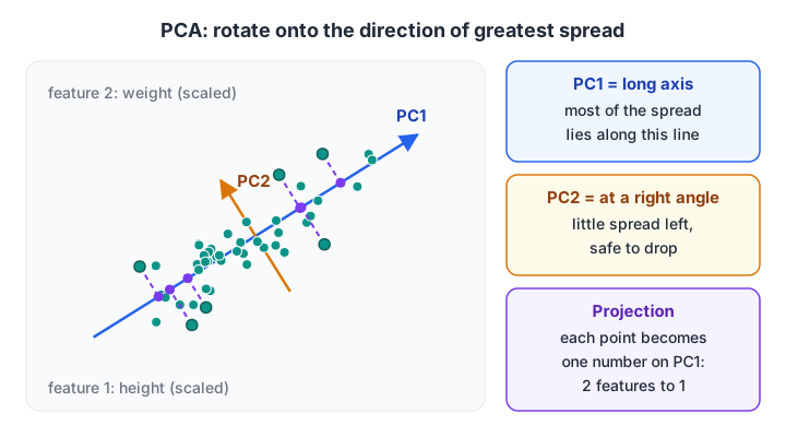
PC1 runs along the direction where the data spreads the most. Projecting each point onto PC1 keeps most of the variation in one number instead of two.
The procedure has five steps:
- Centre the data: subtract each column's mean so the cloud sits at the origin.
- Scale if units differ: divide by the standard deviation so centimetres and kilograms count equally.
- Compute the covariance matrix: a square table of how every pair of features varies together.
- Find its eigenvectors and eigenvalues: each eigenvector is a component direction, and its eigenvalue is the variance along it.
- Project: multiply the centred data by the top k eigenvectors to get k new columns.
Eigenvectors and covariance are covered gently in linear algebra for data science. The code below does all five steps in numpy and checks the answer against scikit-learn.
import numpy as np
from sklearn.decomposition import PCA

rng = np.random.default_rng(7)
size, build = rng.normal(0, 1, (2, 300))
X = np.column_stack([8 * size, 3 * size, 4 * size,
                     4 * size + 6 * build, 3 * size + 7 * build,
                     5 * size + 8 * build]) + rng.normal(0, 1.5, (300, 6))

Z = (X - X.mean(axis=0)) / X.std(axis=0)          # steps 1 and 2
cov = np.cov(Z, rowvar=False)                      # step 3
eigvals, eigvecs = np.linalg.eigh(cov)             # step 4
order = np.argsort(eigvals)[::-1]
eigvals, eigvecs = eigvals[order], eigvecs[:, order]
scores = Z @ eigvecs[:, :2]                        # step 5: keep 2 components

print("variance share per component:", np.round(eigvals / eigvals.sum(), 3))
print("first row in 2D:", np.round(scores[0], 3))

sk = PCA(n_components=2).fit(Z)
print("sklearn explained_variance_ratio_:", np.round(sk.explained_variance_ratio_, 3))
The first two components hold about 94% of the variation in six columns, and the manual numbers match scikit-learn's. A component's sign can flip between implementations; that is harmless, because a direction and its opposite are the same axis.
Each component is a weighted recipe of the original features. Those weights are the loadings, stored in pca.components_, and they help you name a component such as "overall size".
How many principal components should you keep?
The explained variance ratio tells you what fraction of the total variation each component carries. Add them up in order and you get the cumulative curve, often drawn as a scree plot.
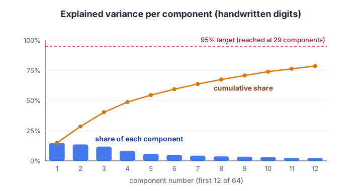
The bars show each component's share of variance. Where the cumulative line crosses your target, usually 90–95%, is a sensible number of components to keep.
The handwritten digits dataset bundled with scikit-learn has 1,797 images of 8×8 pixels, so 64 features per image. Here is how many components it needs:
import numpy as np
from sklearn.datasets import load_digits
from sklearn.decomposition import PCA

X, y = load_digits(return_X_y=True)        # 1797 images, 64 pixel features
pca = PCA().fit(X)
cum = np.cumsum(pca.explained_variance_ratio_)

for target in [0.80, 0.90, 0.95, 0.99]:
    k = int(np.argmax(cum >= target)) + 1
    print(f"{int(target * 100)}% of variance needs {k:2d} of 64 components")

auto = PCA(n_components=0.95).fit(X)       # a float asks for that share of variance
print("PCA(n_components=0.95) kept", auto.n_components_, "components")
Just 21 components keep 90% of the information in 64 pixels. Passing a float between 0 and 1 as n_components lets scikit-learn pick the count for you.
Reconstruction error: what do you lose?
PCA can map compressed data back to the original space with inverse_transform. The gap between the original and the rebuilt rows shows what the dropped components held.
import numpy as np
from sklearn.datasets import load_digits
from sklearn.decomposition import PCA

X, _ = load_digits(return_X_y=True)
for k in [2, 5, 10, 20, 40]:
    pca = PCA(n_components=k).fit(X)
    X_back = pca.inverse_transform(pca.transform(X))
    rmse = np.sqrt(np.mean((X - X_back) ** 2))
    print(f"{k:2d} components -> average pixel error {rmse:.2f} (pixels range 0-16)")
With 20 components the average pixel is off by about 1.4 on a 0–16 scale, and every digit stays readable. The same reconstruction error is also a handy anomaly score, which the anomaly detection tutorial uses next.
Quick check
What does PCA(n_components=0.9) do in scikit-learn?
A float between 0 and 1 is read as a target share of explained variance.
How do you use PCA with scikit-learn in a real model?
In practice, PCA is one pipeline step: scale, reduce, model. Inside a Pipeline, each cross-validation fold fits its own scaler and PCA, so nothing leaks from validation rows. That pattern is explained in cross-validation.
import time
from sklearn.datasets import load_digits
from sklearn.pipeline import make_pipeline
from sklearn.preprocessing import StandardScaler
from sklearn.decomposition import PCA
from sklearn.linear_model import LogisticRegression
from sklearn.model_selection import cross_val_score

X, y = load_digits(return_X_y=True)
for k in [10, 20, 40, None]:            # None keeps all 64 features
    steps = [StandardScaler()] + ([PCA(n_components=k)] if k else [])
    pipe = make_pipeline(*steps, LogisticRegression(max_iter=500))
    t = time.perf_counter()
    acc = cross_val_score(pipe, X, y, cv=3).mean()
    label = k if k else "all 64"
    print(f"features: {label:>6} | accuracy {acc:.3f} | {time.perf_counter() - t:.2f}s")
Forty components score within about a point of all 64 features, and 20 components lose only about three points. On datasets with thousands of columns, the speed gain becomes large. You can tune n_components like any other setting with GridSearchCV, as shown in the hyperparameter tuning tutorial.
Why scaling before PCA matters
PCA chases variance, and variance depends on units. Salary in rupees has a variance in the crores; height in metres, below 1. Unscaled, PC1 simply becomes "salary".
import numpy as np
from sklearn.decomposition import PCA
from sklearn.preprocessing import StandardScaler

rng = np.random.default_rng(1)
height_m = rng.normal(1.65, 0.08, 200)
salary_rs = 30000 + 200000 * (height_m - 1.65) + rng.normal(0, 8000, 200)
X = np.column_stack([height_m, salary_rs])

raw = PCA(n_components=1).fit(X)
scaled = PCA(n_components=1).fit(StandardScaler().fit_transform(X))
print("PC1 loadings without scaling:", np.round(raw.components_[0], 4))
print("PC1 loadings with scaling:   ", np.round(scaled.components_[0], 4))
Unscaled, height gets a loading of zero despite its strong link to salary. Scaled, both features contribute equally. Scaling methods are compared in the data preprocessing tutorial on scaling and encoding.
Quick check
You run PCA on columns for salary (rupees) and age (years) without scaling. What happens?
PCA ranks directions by variance, which depends on units. Standardise first so each column has unit variance.
PCA vs other dimensionality reduction techniques
PCA is linear. For curved or clustered structure, other tools do better.
| Method | Type | Best for | Watch out for |
|---|---|---|---|
| PCA | Linear, unsupervised | Compressing correlated numeric features, speeding up models | Needs scaling; components are hard to name |
| TruncatedSVD | Linear, unsupervised | Sparse data such as TF-IDF text matrices | No centring, so variance shares differ from PCA |
| Linear Discriminant Analysis | Linear, supervised | Reducing features while keeping classes apart | At most (classes − 1) components |
| t-SNE | Non-linear | 2D visualisation of clusters | Distances between clusters are not meaningful; slow |
| UMAP | Non-linear | Visualisation and fast embeddings | Separate library; results depend on settings |
| Autoencoder | Non-linear, neural | Images, very large or complex data | Needs a deep learning framework and more data |
| Feature selection | Keeps original columns | When you must explain which inputs matter | Does not combine information across columns |
If stakeholders need to know which original column drives a prediction, prefer feature selection, because PCA's components are blends. Autoencoders, covered in the deep learning series, are the neural version of this compression.
Common PCA mistakes
- Skipping scaling when columns use different units. The biggest-unit column takes over PC1.
- Fitting PCA on all data before splitting. That leaks test information. Fit inside a pipeline.
- Using PCA before tree models by default. Trees such as random forests handle many correlated features well, and rotated features can make their splits worse.
- Keeping too few components because a 2D plot looks nice. Check cumulative variance and the model score.
Turning theory like this into habit takes repetition on messy datasets, which is where classroom machine learning training at Debugshala's Indore campus helps. For quick revision, try PCA and linear algebra MCQs on Debugshala Test.
Key takeaways
- PCA replaces many correlated features with a few uncorrelated components ranked by variance.
- The steps are centre, scale, covariance, eigenvectors, project.
- Use the cumulative explained variance (scree plot) to choose how many components to keep, typically 90–95%.
inverse_transformshows what you lost; reconstruction error doubles as an anomaly score.- Always scale first and fit PCA inside a Pipeline.
- PCA is linear and unsupervised; use t-SNE or UMAP for visual clusters and feature selection when you need named inputs.
FAQ
What is PCA used for in machine learning?
PCA is used to reduce the number of features while keeping most of the information. Typical uses are faster training, removing multicollinearity before linear models, compressing image or sensor data, denoising, and plotting high-dimensional data in two or three dimensions.
Is PCA supervised or unsupervised?
PCA is unsupervised. It looks only at the input features and how they vary together, never at the target labels. That is why PCA can throw away a low-variance direction that happens to be useful for prediction. Linear Discriminant Analysis is the supervised alternative that uses class labels.
Should I standardise data before PCA?
Yes, whenever features are in different units or scales. PCA ranks directions by variance, so a column measured in rupees will swamp one measured in years. Standardising each feature to mean 0 and standard deviation 1 lets every feature compete fairly. Skip it only when all features share one meaningful unit.
How many components should I keep in PCA?
Keep the smallest number that explains about 90–95% of the variance, then confirm with cross-validated model performance. For visualisation you keep two or three regardless. If a model scores the same with 20 components as with 64 features, the smaller version is usually the better choice.
Where can I learn PCA and unsupervised learning in Indore?
Debugshala, a training and placement institute in Indore, runs a Machine Learning course at its Old Palasia campus, with classes in English and Hindi. Fresh graduates, non-IT learners and people with a year gap can join, and a free demo class is available before you pay.
From the team behind this site
Go further with the Data Science & AI Course at Debugshala
These tutorials are written by Debugshala, a training and placement institute at Old Palasia, Indore. The classroom course adds live mentoring, real projects and interview preparation.
- Offline classes at Old Palasia, Indore
- Free demo class before you pay
- Non-IT, fresher and year-gap friendly
- Placement assistance
700+ students placed · 200+ hiring partners · 4.9★ Google rating
