

Linear Algebra for Data Science: Vectors, Matrices, Python
Linear algebra for data science made practical: vectors, dot products, cosine similarity, matrix multiplication and eigenvectors, with runnable numpy code.
Think of a mobile shop on MG Road that sells three phone models. On Monday it sold 4, 2 and 1 units. The prices are ₹12,000, ₹18,000 and ₹30,000. To get Monday's revenue you multiply each count by its price and add the results: 4 × 12,000 + 2 × 18,000 + 1 × 30,000 = ₹1,14,000.
Now the owner wants revenue for all seven days of the week. You write the seven rows of counts one below the other and repeat the same "multiply and add" for each row. That single repeated operation is matrix multiplication, and you just did linear algebra without the name.
A linear regression model does the same thing, except it learns the weights from history instead of reading them off a price tag.
What is linear algebra in data science?
Map the shop to the vocabulary:
- One day's sales, [4, 2, 1], is a vector: an ordered list of numbers.
- The seven days stacked together form a matrix with 7 rows and 3 columns, written 7 × 3.
- The prices, [12000, 18000, 30000], are a weight vector.
- "Multiply matching entries and add" is the dot product.
Linear algebra is the branch of mathematics that works with vectors and matrices, and data science uses it to represent datasets as matrices and to express models, distances and transformations as operations on them.
After probability and sampling techniques, this is the last maths topic in the series, and you don't have to compute any of it by hand. numpy, the open-source Python library for numerical arrays, does it in compiled code. If arrays are new to you, read NumPy arrays explained first. This article targets Python 3.12+ and numpy 1.26 or newer.
import numpy as np

monday = np.array([4, 2, 1])               # units of phone A, B, C
prices = np.array([12000, 18000, 30000])   # rupees per unit

print("Monday revenue:", monday @ prices)  # @ is the dot product here
print("Same thing, by hand:", (monday * prices).sum())

week = np.array([[4, 2, 1], [3, 3, 0], [5, 1, 2], [2, 2, 2],
                 [6, 4, 1], [8, 5, 3], [7, 3, 2]])
print("Shape of the week matrix:", week.shape)
print("Revenue per day:", week @ prices)
Vectors: one row of data as an arrow
A vector with two numbers can be drawn as an arrow on graph paper. A vector with 30 numbers can't be drawn, but the same rules apply. Every row in your dataset is a point in a space with one dimension per column.
Two measurements describe a vector:
- Its length (also called the norm): the square root of the sum of squared entries. For [3, 4] the length is 5.
- Its direction: where it points, regardless of length.
Adding vectors works entry by entry, and multiplying by a number (a scalar) stretches or shrinks them. These two moves are what "linear" means.
Distance between two rows
The distance between two customers is the length of the difference of their vectors. This is the Euclidean distance that k-nearest neighbors and k-means clustering depend on.
import numpy as np

# age, monthly spend in thousands, visits per month
asha  = np.array([24, 3.5, 6])
ravi  = np.array([26, 4.0, 5])
meena = np.array([58, 1.0, 1])

print("Length of Asha's vector:", round(np.linalg.norm(asha), 2))
print("Asha to Ravi :", round(np.linalg.norm(asha - ravi), 2))
print("Asha to Meena:", round(np.linalg.norm(asha - meena), 2))
Asha sits much closer to Ravi than to Meena. Notice, though, that age dominates the distance because its numbers are bigger. That is why distance-based models need scaling first.
What does the dot product tell you?
The dot product of two vectors multiplies matching entries and adds them up. It has two uses you will meet again and again.
First, it is a weighted sum. Revenue was counts · prices. A linear model's prediction is features · weights + bias.
Second, it measures how much two vectors point the same way. Divide the dot product by both lengths and you get the cosine of the angle between them, called cosine similarity. It runs from −1 (opposite) through 0 (unrelated) to 1 (same direction).
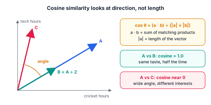
Cosine similarity ignores length and looks only at the angle, so a heavy reader and a light reader with the same tastes score close to 1.
Cosine similarity is how search engines, recommender systems and text embeddings decide that two items are alike.
import numpy as np

# Hours a user spent on: cricket, finance, cooking, tech news
user_a = np.array([10, 2, 0, 6])
user_b = np.array([5, 1, 0, 3])     # same taste, half the time
user_c = np.array([0, 1, 9, 0])

def cosine(u, v):
    return (u @ v) / (np.linalg.norm(u) * np.linalg.norm(v))

print("A vs B:", round(cosine(user_a, user_b), 3))
print("A vs C:", round(cosine(user_a, user_c), 3))
User B spends half the time but has an identical profile, so the score is 1.0. Choosing the similarity measure is a modelling decision, not a detail.
Quick check
Two users have profiles [2, 4, 0] and [4, 8, 0]. What is their cosine similarity?
The second vector is exactly twice the first, so they point in the same direction and the cosine is 1.
Matrices and matrix multiplication
A matrix is a grid of numbers with a shape of rows × columns. In data science the usual convention is: rows are observations, columns are features. A dataset of 1,000 houses with 5 features is a 1000 × 5 matrix, usually called X.
Matrix multiplication takes each row of the first matrix and dots it with each column of the second. For it to work, the inner sizes must match: (7 × 3) times (3 × 1) gives 7 × 1. Read the rule as "the 3s cancel".
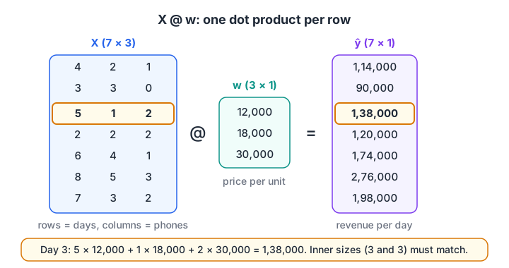
Every prediction is one row of X dotted with the weight vector, so one matrix product scores the whole table.
Three facts save beginners hours of confusion:
- Order matters. A @ B is usually not equal to B @ A, and often only one of them is even allowed.
A * Bin numpy is element-wise multiplication, not matrix multiplication. Use@ornp.matmulfor the real thing.- The transpose, written Aᵀ and
A.Tin numpy, flips rows and columns. It shows up whenever you need the shapes to line up.
Linear regression is one matrix equation
Fitting a line by least squares has a closed-form answer: w = (XᵀX)⁻¹ Xᵀy. The formula shows that linear regression is nothing more than matrix arithmetic.
import numpy as np

rng = np.random.default_rng(1)
n = 200
area = rng.uniform(600, 2000, n)             # square feet
age = rng.uniform(0, 30, n)                  # years
price = 15 + 0.04 * area - 0.6 * age + rng.normal(0, 3, n)  # lakhs

X = np.column_stack([np.ones(n), area, age])  # column of 1s = intercept
w, *_ = np.linalg.lstsq(X, price, rcond=None)  # stable least squares
print("Intercept, per sq ft, per year:", w.round(3))

new_flats = np.array([[1, 1200, 5], [1, 900, 20]])
print("Predicted prices (lakhs):", (new_flats @ w).round(1))
The recovered weights land close to the true 15, 0.04 and −0.6. Prefer lstsq over np.linalg.inv: inverting is slower and fragile when columns are nearly duplicates.
Quick check
X has shape (500, 8) and w has shape (8,). What is the shape of X @ w?
The inner dimension 8 cancels, leaving one prediction for each of the 500 rows.
Eigenvalues and eigenvectors, without the fear
Most matrices rotate and stretch the vectors they multiply. An eigenvector is a special direction that the matrix only stretches, never turns. The stretch factor is its eigenvalue.
Why care? Take the covariance matrix of your data, which records how every pair of columns varies together. Its eigenvectors point along the directions where the data spreads the most, and the eigenvalues say how much spread each direction holds. That is the entire idea behind principal component analysis.
import numpy as np

rng = np.random.default_rng(0)
study_hours = rng.normal(5, 2, 300)
marks = 8 * study_hours + rng.normal(0, 6, 300)    # strongly related
data = np.column_stack([study_hours, marks])

cov = np.cov(data, rowvar=False)
values, vectors = np.linalg.eigh(cov)              # eigh: for symmetric matrices
order = values.argsort()[::-1]
share = values[order] / values.sum()
print("Variance explained by each direction:", share.round(3))
print("Main direction (eigenvector):", vectors[:, order[0]].round(3))
One direction holds almost all the variance, because marks and hours move together. PCA would say this two-column dataset is really about one thing.
Which linear algebra topics matter for which models?
| Concept | Where you meet it | numpy |
|---|---|---|
| Vector norm, distance | KNN, k-means, outlier scores | np.linalg.norm |
| Dot product | Linear and logistic regression, neural network layers | a @ b |
| Cosine similarity | Search, recommendations, embeddings | a @ b / (norm·norm) |
| Matrix multiplication | Scoring a whole dataset, every neural layer | X @ W |
| Transpose, inverse, least squares | Regression formulas | X.T, np.linalg.lstsq |
| Eigen decomposition | PCA, covariance analysis | np.linalg.eigh |
| Rank, near-duplicate columns | Multicollinearity warnings | np.linalg.matrix_rank |
If you want a structured way to learn this alongside regression and PCA, the maths-backed data science course at Debugshala builds these ideas into model-building from the first weeks.
Common mistakes with linear algebra in Python
- Using
*when you meant@. Element-wise and matrix multiplication give different shapes and different answers. - Mixing up shape (3,) and (3, 1). A 1-D array and a column vector broadcast differently. Print
.shapewhenever a result looks odd. - Inverting matrices directly. Prefer
np.linalg.solveorlstsq. They are faster and more stable. - Forgetting the intercept column. Without a column of ones, your regression line is forced through zero.
- Comparing unscaled vectors. A column measured in rupees will swamp a column measured in years.
Key takeaways
- A dataset is a matrix: rows are observations, columns are features.
- The dot product is both a weighted sum and a similarity score.
- Matrix multiplication applies the same weights to every row at once; the inner shapes must match.
- Least squares regression is a single matrix equation, solved stably with
lstsq. - Eigenvectors of the covariance matrix are the directions of greatest spread, which is what PCA keeps.
- Scaling matters because distances and dot products are dominated by large-valued columns.
With probability, inference and now linear algebra in place, the series moves on to working with real data, starting with exploratory data analysis. To check your shape rules and dot products under time pressure, solve matrix and vector MCQs on Debugshala Test.
FAQ
How much linear algebra do I need for data science?
You need vectors, dot products, matrix multiplication, transpose, norms and a working idea of eigenvectors. That covers regression, distance-based models, PCA and how neural network layers compute. Proof techniques and abstract vector spaces are not required for most data science jobs, though they help in research roles.
Is linear algebra or calculus more important for machine learning?
For everyday data science, linear algebra comes up more often, because every dataset and model is stored and computed as matrices. Calculus matters for understanding how models are trained, especially gradient descent. Learn linear algebra first, then the derivative and the chain rule when you reach neural networks.
What is the difference between a vector and a matrix?
A vector is a one-dimensional list of numbers, such as one customer's features. A matrix is a two-dimensional grid, such as a whole table of customers. In numpy a vector usually has shape (n,) and a matrix has shape (rows, columns).
Why is cosine similarity used instead of distance?
Cosine similarity compares direction and ignores length, so it judges two items by their pattern rather than their size. A short and a long document on the same topic score as similar. Euclidean distance would call them far apart because one vector is longer.
Can I learn linear algebra for data science in Indore?
Yes. Debugshala, a training and placement institute at Old Palasia, Indore, teaches the linear algebra needed for machine learning inside its Data Science & AI course. Classes run offline and online in English and Hindi. You can attend a free demo class before paying, and non-IT graduates are welcome.
From the team behind this site
Go further with the Data Science & AI Course at Debugshala
These tutorials are written by Debugshala, a training and placement institute at Old Palasia, Indore. The classroom course adds live mentoring, real projects and interview preparation.
- Offline classes at Old Palasia, Indore
- Free demo class before you pay
- Non-IT, fresher and year-gap friendly
- Placement assistance
700+ students placed · 200+ hiring partners · 4.9★ Google rating
