

Bayes' Theorem Explained with Examples and Python Code
Bayes' theorem made intuitive with a dengue test example, natural frequency trees, spam filtering and Bayesian A/B testing, each with runnable Python.
It is August in Indore and dengue cases are in the news. You feel a bit feverish, go to a lab and take a rapid test. It comes back positive. The lab says the test catches 90% of real dengue cases.
Most people now assume they have a 90% chance of dengue. That feels right, and it is badly wrong. If only 2 in 100 people with a mild fever actually have dengue, your real chance after one positive test is closer to 27%.
The gap between 90% and 27% is the reason Bayes' theorem exists. It forces you to combine what the test says with how common the condition was to begin with.
What is Bayes' theorem?
Map the lab visit to the terms:
- "I have dengue" is the hypothesis H.
- "The test is positive" is the evidence E.
- 2% of feverish patients having dengue is the prior, P(H), your belief before the test.
- The test catching 90% of real cases is the likelihood, P(E | H).
- Your chance of dengue after the positive result is the posterior, P(H | E).
Bayes' theorem is a formula for reversing a conditional probability: it computes P(H | E) from P(E | H), the prior P(H) and the overall chance of the evidence P(E).
P(H | E) = P(E | H) × P(H) / P(E)
The bottom part, P(E), is the total chance of seeing a positive test from anyone, sick or healthy. You get it by adding both routes to a positive result: P(E) = P(E | H) × P(H) + P(E | not H) × P(not H).
The probability for data science tutorial showed that P(late | rain) and P(rain | late) are different numbers. Bayes' theorem is the bridge between the two.
The dengue test, worked with natural frequencies
Formulas with Greek letters lose most people. Counting people does not. Imagine 10,000 feverish patients and follow them through the test.
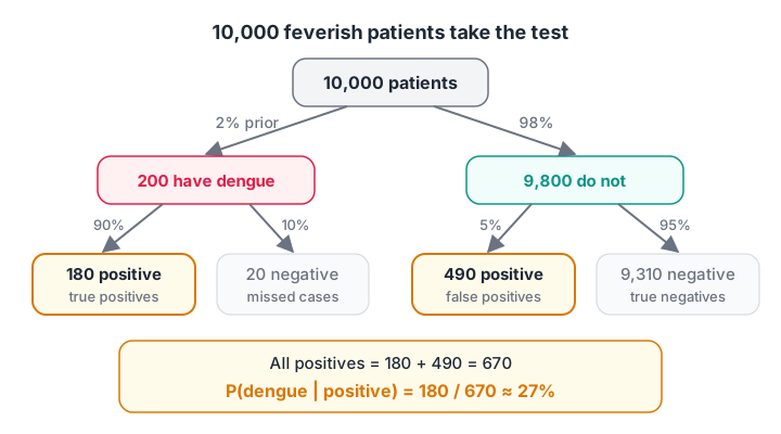
Out of 670 positive results, only 180 belong to people who really have dengue, so P(dengue | positive) = 180 / 670, about 27%.
The numbers we assumed:
| Quantity | Value | Meaning |
|---|---|---|
| Prior P(dengue) | 0.02 | 2% of feverish patients have dengue |
| Sensitivity P(+ given dengue) | 0.90 | test catches 90% of real cases |
| False positive rate P(+ given no dengue) | 0.05 | 5% of healthy people still test positive |
Follow the tree step by step:
- Of 10,000 patients, 2% (200) have dengue and 9,800 do not.
- Of the 200 with dengue, 90% test positive: 180 true positives.
- Of the 9,800 without dengue, 5% test positive: 490 false positives.
- Total positives: 180 + 490 = 670.
- Share of positives who really have dengue: 180 / 670 ≈ 0.27.
The healthy group is so much bigger that even a small false positive rate swamps the true cases. This trap has a name: the base rate fallacy.
def bayes(prior, p_e_given_h, p_e_given_not_h):
    evidence = p_e_given_h * prior + p_e_given_not_h * (1 - prior)
    return p_e_given_h * prior / evidence

posterior = bayes(prior=0.02, p_e_given_h=0.90, p_e_given_not_h=0.05)
print(f"P(dengue | positive test) = {posterior:.3f}")

# Same answer by counting 10,000 people
sick, healthy = 10_000 * 0.02, 10_000 * 0.98
tp, fp = sick * 0.90, healthy * 0.05
print(f"True positives {tp:.0f}, false positives {fp:.0f}, share = {tp / (tp + fp):.3f}")
Checking the answer by simulation
If the result still feels wrong, simulate a population and count. This is a good habit for any probability result that surprises you.
import numpy as np

rng = np.random.default_rng(11)
n = 200_000
has_dengue = rng.random(n) < 0.02

# Positive with prob 0.90 if sick, 0.05 if healthy
p_positive = np.where(has_dengue, 0.90, 0.05)
test_positive = rng.random(n) < p_positive

print("Patients who tested positive:", test_positive.sum())
print("Of those, truly sick:", (has_dengue & test_positive).sum())
print(f"P(dengue | positive) by simulation: {has_dengue[test_positive].mean():.3f}")
Prior, likelihood and posterior: how beliefs update
Bayes' theorem is not a one-off calculation. Today's posterior becomes tomorrow's prior. Each new piece of evidence nudges the belief further.
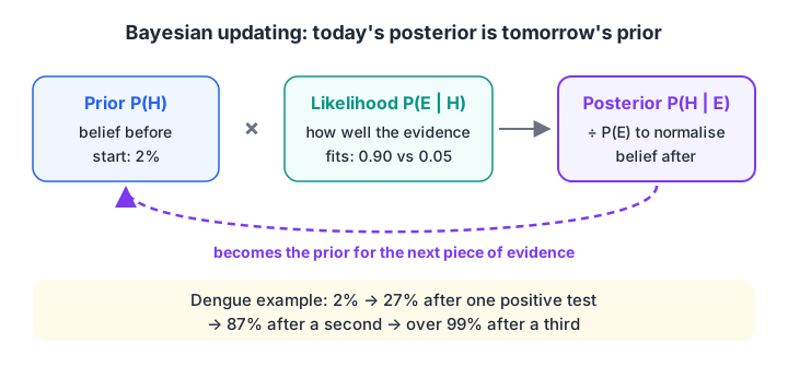
Each test result updates the belief, and the posterior from one step becomes the prior for the next.
Suppose the doctor orders a second, independent test, and it is also positive. Your prior for the second test is no longer 2%. It is the 27% you just calculated.
def bayes(prior, p_e_given_h, p_e_given_not_h):
    evidence = p_e_given_h * prior + p_e_given_not_h * (1 - prior)
    return p_e_given_h * prior / evidence

belief = 0.02
print(f"Before any test:      {belief:.3f}")
for i in range(1, 4):
    belief = bayes(belief, 0.90, 0.05)
    print(f"After positive test {i}: {belief:.3f}")
Two positives take you from 2% to about 87%. A third pushes you above 99%. This is why doctors confirm surprising results with a second test rather than acting on the first.
The order of the evidence does not matter, but its independence does. Two tests that share the same flaw, such as reacting to a related virus, are not independent, and multiplying their evidence would overstate your confidence.
Quick check
In Bayes' theorem, which term is your belief before seeing the evidence?
The prior P(H) is the starting belief. The posterior P(H | E) is the updated belief after the evidence.
Bayes' theorem in data science
The same three ingredients appear across data work.
Spam and fraud filters
Replace "dengue" with "spam" and "positive test" with "email contains the word free". Estimate the prior from the share of spam in your inbox, and the likelihoods from how often free appears in spam and in normal mail.
import pandas as pd

emails = pd.DataFrame({
    "is_spam":  [1]*30 + [0]*70,
    "has_free": [1]*12 + [0]*18 + [1]*4 + [0]*66,
})

prior = emails.is_spam.mean()
p_free_spam = emails.loc[emails.is_spam == 1, "has_free"].mean()
p_free_ham = emails.loc[emails.is_spam == 0, "has_free"].mean()

evidence = p_free_spam * prior + p_free_ham * (1 - prior)
print(f"Prior P(spam)        = {prior:.2f}")
print(f"P('free' | spam)     = {p_free_spam:.2f},  P('free' | not spam) = {p_free_ham:.3f}")
print(f"P(spam | 'free')     = {p_free_spam * prior / evidence:.2f}")
A real filter combines hundreds of words this way, assuming they are independent. That model is the Naive Bayes classifier, one of the fastest text classifiers you can train.
Bayesian A/B testing
In an experiment, the hypothesis is "the true conversion rate is p". You start with a prior over all possible values of p, then update it with the clicks you observe. A simple grid approximation does this with plain numpy: try every p from 0 to 1, multiply prior by likelihood, and normalise.
import numpy as np
from math import comb

p_grid = np.linspace(0, 1, 1001)
prior = np.ones_like(p_grid)                   # flat prior: every rate equally likely

visitors, signups = 200, 18
likelihood = comb(visitors, signups) * p_grid**signups * (1 - p_grid)**(visitors - signups)
posterior = prior * likelihood
posterior /= posterior.sum()

mean = (p_grid * posterior).sum()
cdf = posterior.cumsum()
low, high = p_grid[np.searchsorted(cdf, 0.025)], p_grid[np.searchsorted(cdf, 0.975)]
print(f"Posterior mean conversion rate: {mean:.3f}")
print(f"95% credible interval: {low:.3f} to {high:.3f}")
print(f"P(rate > 12%): {posterior[p_grid > 0.12].sum():.3f}")
With 200 visitors the credible interval is wide, just as the central limit theorem would predict for a small sample. The result is also a direct probability statement, such as "there is about a 10% chance the rate exceeds 12%."
Many product teams find that easier to act on than a p-value. The A/B testing tutorial covers the classical approach in detail.
Quick check
A fraud model flags 95% of fraudulent transactions and wrongly flags 2% of genuine ones. Fraud is 0.1% of all transactions. Roughly what share of flagged transactions are fraud?
Per 100,000 transactions: 95 frauds flagged and about 1,998 genuine ones flagged. 95 / 2,093 is about 4.5%.
Common mistakes with Bayes' theorem
- Ignoring the prior. A highly accurate test for a rare event still gives mostly false alarms. Always ask how common the thing is.
- Confusing P(E | H) with P(H | E). "90% of dengue patients test positive" is not "90% of positives have dengue."
- Forgetting false positives in the denominator. P(E) includes everyone who could produce the evidence, not only the true cases.
- Treating correlated evidence as independent. Updating twice on the same underlying signal double-counts it.
- Using a prior of exactly 0 or 1. No amount of evidence can move a belief that starts at certainty.
Key takeaways
- Bayes' theorem reverses a conditional probability: P(H | E) = P(E | H) × P(H) / P(E).
- Posterior = likelihood × prior ÷ evidence; the evidence term adds up every route to the observation.
- Counting a population of 10,000 makes any Bayes problem intuitive.
- Rare conditions plus imperfect tests mean many false positives: the base rate fallacy.
- Posteriors become priors, so repeated independent evidence builds confidence quickly.
- Spam filters, fraud alerts and Bayesian A/B tests all use the same formula.
The next topic, hypothesis testing, takes the classical route to deciding whether evidence is strong enough. To practise problems like the fraud question above, attempt probability quizzes on Debugshala Test.
FAQ
What is Bayes' theorem in simple words?
Bayes' theorem is a rule for updating a belief when you get new evidence. You start with how likely something was before (the prior), weigh how well the evidence fits it compared with the alternatives, and end with an updated probability (the posterior). It is how you should change your mind, in numbers.
Why is Bayes' theorem important in machine learning?
It underlies the Naive Bayes classifier, Bayesian networks, Bayesian hyperparameter optimisation and probabilistic models in general. Even models that do not use it directly, such as logistic regression, are often explained through the prior and likelihood. It also gives a principled way to add domain knowledge through the prior.
What is the difference between likelihood and probability?
Probability asks how likely the data is for a fixed hypothesis. Likelihood takes the observed data as fixed and asks how well each possible hypothesis explains it. In Bayes' theorem, P(E | H) is read as the likelihood of H given the evidence, even though it is written as a probability of E.
What is the base rate fallacy?
The base rate fallacy is ignoring how common something is when judging evidence about it. A test with 90% sensitivity sounds conclusive, but if only 2% of people have the condition, false positives from the healthy 98% can outnumber true positives. Bayes' theorem corrects this by putting the base rate in as the prior.
Is Bayes' theorem taught in data science courses in Indore?
Yes. Debugshala, an industry-aligned training and placement institute at Old Palasia, Indore, includes probability and Bayes' theorem in its Data Science & AI course. You can study offline at the campus or online, in English or Hindi, and attend a free demo class first. Explore the Old Palasia data science classroom programme for details.
From the team behind this site
Go further with the Data Science & AI Course at Debugshala
These tutorials are written by Debugshala, a training and placement institute at Old Palasia, Indore. The classroom course adds live mentoring, real projects and interview preparation.
- Offline classes at Old Palasia, Indore
- Free demo class before you pay
- Non-IT, fresher and year-gap friendly
- Placement assistance
700+ students placed · 200+ hiring partners · 4.9★ Google rating
