

Hypothesis Testing in Python: p-values, t-tests, Chi-square
Hypothesis testing step by step: null and alternative, p-values, Welch's t-test, chi-square and Type I/II errors, with numpy code that runs in your browser.
An Indore coaching centre tries a new revision method with one batch of 12 students and keeps the old method for another batch of 12. On the next mock test, the new batch averages 67.5 and the old batch averages 61.
The director is ready to switch every batch. A teacher asks a fair question: "Students' scores jump around by five or six marks anyway. Could a 6.5-mark gap happen just by luck?"
Hypothesis testing is the formal way to answer that teacher. It does not tell you the method works. It tells you how hard it would be to see a gap this big if the method did nothing.
What is hypothesis testing?
Map the coaching story to the terms:
- "The new method makes no difference" is the null hypothesis, H₀.
- "The new method changes scores" is the alternative hypothesis, H₁.
- The 6.5-mark gap, scaled by the noise, is the test statistic.
- How often a gap this large would appear if H₀ were true is the p-value.
- The cut-off you agreed on in advance, usually 0.05, is the significance level, α.
Hypothesis testing is a statistical procedure that measures how compatible sample data is with a null hypothesis, and rejects that null when the data would be too unlikely under it.
It works like a court case. The null hypothesis is "innocent until proven guilty." You only reject it when the evidence is strong. Failing to reject is not the same as proving innocence; it just means the evidence was not enough.
The five steps of a hypothesis test
- State the hypotheses. H₀: mean score is the same for both methods. H₁: the means differ.
- Choose α before looking at the data. 0.05 is common; medicine often uses stricter values.
- Pick the test and compute the statistic. For two group means, a t-test.
- Find the p-value. The probability, under H₀, of a statistic at least as extreme as yours.
- Decide and report. If p < α, reject H₀. Report the effect size and a confidence interval, not just the p-value.
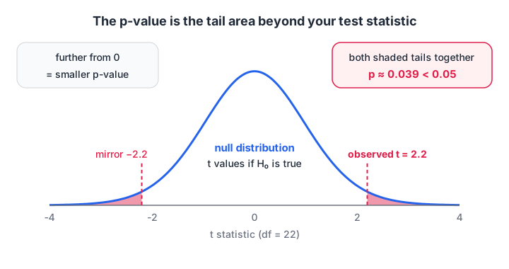
The curve shows test statistics you would expect if H₀ were true; the p-value is the area beyond your observed value in both tails.
The curve comes from the central limit theorem: differences in sample means are approximately normal, and with estimated standard deviations they follow a t distribution.
The t-test: comparing means
What does a t statistic measure?
A t statistic is signal divided by noise. The signal is the difference in means. The noise is the standard error of that difference, which depends on how spread out each group is and how many students it has.
t = (mean₂ − mean₁) / √(s₁² / n₁ + s₂² / n₂)
This version, which does not assume both groups have equal variance, is Welch's t-test. It is the safer default.
scipy is not available in the browser sandbox, so the block below computes the two-sided p-value by integrating the t distribution's density with numpy. The t_pvalue helper is only a few lines and gives the same answer scipy would.
import numpy as np
from math import gamma, pi, sqrt

def t_pvalue(t, df):
    x = np.linspace(-abs(t), abs(t), 40001)
    pdf = gamma((df + 1) / 2) / (sqrt(df * pi) * gamma(df / 2)) * (1 + x**2 / df) ** (-(df + 1) / 2)
    return 1 - np.sum((pdf[1:] + pdf[:-1]) / 2 * np.diff(x))   # area outside -|t|..|t|

old = np.array([58, 62, 55, 67, 60, 64, 59, 61, 57, 66, 63, 60])
new = np.array([65, 70, 61, 72, 66, 63, 69, 74, 64, 68, 71, 67])

v1, v2, n1, n2 = old.var(ddof=1), new.var(ddof=1), len(old), len(new)
se = sqrt(v1 / n1 + v2 / n2)
t = (new.mean() - old.mean()) / se
df = (v1/n1 + v2/n2) ** 2 / ((v1/n1) ** 2 / (n1 - 1) + (v2/n2) ** 2 / (n2 - 1))

print(f"Means: old={old.mean():.1f}, new={new.mean():.1f}, gap={new.mean() - old.mean():.1f}")
print(f"t = {t:.2f}, Welch df = {df:.1f}, p-value = {t_pvalue(t, df):.5f}")
diff = new.mean() - old.mean()
print(f"Approx. 95% CI for the gap: {diff - 2.07*se:.1f} to {diff + 2.07*se:.1f} marks")
The p-value is about 0.0003. If the method truly did nothing, a gap this large would show up roughly 3 times in 10,000 repeats. You reject H₀. The confidence interval (about 3 to 10 marks) tells you how big the improvement plausibly is. The 2.07 multiplier is the t critical value for about 22 degrees of freedom.
On your own machine with scipy installed, the same test is one line:
import numpy as np
from scipy import stats

old = np.array([58, 62, 55, 67, 60, 64, 59, 61, 57, 66, 63, 60])
new = np.array([65, 70, 61, 72, 66, 63, 69, 74, 64, 68, 71, 67])

result = stats.ttest_ind(new, old, equal_var=False)   # Welch's t-test
print(result.statistic, result.pvalue)

# One-sample test against a target value (weights from the next example)
# stats.ttest_1samp(weights, popmean=50)
One-sample t-test
Sometimes you compare one group to a fixed target. A namkeen brand prints "50 g" on its packets. A quality check weighs 15 packets. Are they under-filled, or is the shortfall just noise?
import numpy as np
from math import gamma, pi, sqrt

def t_pvalue(t, df):
    x = np.linspace(-abs(t), abs(t), 40001)
    pdf = gamma((df + 1) / 2) / (sqrt(df * pi) * gamma(df / 2)) * (1 + x**2 / df) ** (-(df + 1) / 2)
    return 1 - np.sum((pdf[1:] + pdf[:-1]) / 2 * np.diff(x))

weights = np.array([49.2, 50.1, 48.7, 49.5, 50.3, 48.9, 49.8, 49.1,
                    50.0, 48.6, 49.4, 49.7, 48.8, 49.9, 49.3])
n = len(weights)
t = (weights.mean() - 50) / (weights.std(ddof=1) / sqrt(n))

print(f"Mean weight = {weights.mean():.2f} g from {n} packets")
print(f"t = {t:.2f}, df = {n - 1}, p-value = {t_pvalue(t, n - 1):.4f}")
The packets average 49.42 g and p is below 0.001. The shortfall is small but consistent, so it is unlikely to be chance.
A permutation test: no formulas needed
If you are unsure about the t-test's assumptions, a permutation test answers the same question by brute force. If the method made no difference, the "old" and "new" labels are arbitrary. So shuffle the labels thousands of times and see how often a shuffled gap beats the real one.
import numpy as np

rng = np.random.default_rng(0)
old = np.array([58, 62, 55, 67, 60, 64, 59, 61, 57, 66, 63, 60])
new = np.array([65, 70, 61, 72, 66, 63, 69, 74, 64, 68, 71, 67])
observed = new.mean() - old.mean()

pooled = np.concatenate([old, new])
gaps = []
for _ in range(20_000):
    rng.shuffle(pooled)
    gaps.append(pooled[12:].mean() - pooled[:12].mean())

p = np.mean(np.abs(gaps) >= abs(observed))
print(f"Observed gap: {observed:.1f}  |  permutation p-value: {p:.4f}")
The permutation p-value (about 0.001) is close to the t-test's 0.0003, and both lead to the same decision. Permutation tests are a great way to understand what a p-value means, because you literally build the "world where H₀ is true" and look at it.
The chi-square test: are two categories related?
t-tests compare numbers. When both variables are categories, such as "lead source" and "enrolled or not", you use a chi-square test of independence.
The idea: if lead source and enrolment were unrelated, each source would enrol at the overall rate. The test compares the observed counts with those expected counts and adds up (observed − expected)² / expected across every cell.
import numpy as np
from math import exp

# rows: Instagram, Google, Referral   cols: enrolled, not enrolled
observed = np.array([[30, 120],
                     [45, 105],
                     [40,  60]])

row_tot = observed.sum(axis=1, keepdims=True)
col_tot = observed.sum(axis=0, keepdims=True)
expected = row_tot * col_tot / observed.sum()

chi2 = ((observed - expected) ** 2 / expected).sum()
dof = (observed.shape[0] - 1) * (observed.shape[1] - 1)
p = exp(-chi2 / 2)          # exact chi-square tail formula when dof = 2

print("Expected counts:\n", expected.round(1))
print(f"chi-square = {chi2:.2f}, dof = {dof}, p-value = {p:.5f}")
print("Enrolment rate by source:", (observed[:, 0] / row_tot.ravel()).round(2))
Referral leads enrol at 40% while Instagram leads enrol at 20%. The p-value is well below 0.05, so lead source and enrolment are very unlikely to be independent. With scipy you would call stats.chi2_contingency(observed). Expect each expected count to be at least 5 for the test to be reliable.
Quick check
You want to know whether payment method (UPI, card, cash) is related to whether an order is returned. Which test fits?
Both variables are categorical, so you compare observed and expected counts in a contingency table with a chi-square test.
Type I and Type II errors
Any decision made from a sample can be wrong in two ways.
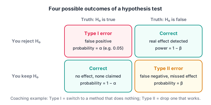
α controls how often you raise false alarms; power (1 − β) is how often you catch a real effect.
| H₀ is actually true | H₀ is actually false | |
|---|---|---|
| Reject H₀ | Type I error (false positive), probability α | Correct: real effect found (power) |
| Fail to reject H₀ | Correct | Type II error (false negative), probability β |
Lowering α to 0.01 cuts false alarms but makes you miss more real effects. The only way to reduce both is more data. Planning a sample size so that power reaches 80% is a core part of A/B testing.
Quick check
Rejecting a true null hypothesis is called what?
A Type I error is a false positive. Its probability is the significance level alpha.
Common mistakes in hypothesis testing
- Reading p as P(H₀ is true). A p-value assumes H₀ is true and asks how surprising the data is. For the probability of a hypothesis, you need Bayes' theorem.
- Treating p = 0.049 and p = 0.051 as opposites. They are nearly the same evidence. Report the number, not just "significant".
- Ignoring effect size. With 1 million rows, a 0.01-mark difference can be "significant" and still useless.
- Running many tests and reporting the winners. Test 20 unrelated features at α = 0.05 and about one will look significant by chance. Correct for multiple comparisons.
- Choosing the test after peeking. Decide the hypothesis, test and α before you see the result.
- Using Student's t-test with unequal variances. Welch's version is the safer default.
If you also work in R, the R hypothesis testing tutorial shows the same tests with t.test() and chisq.test(). For a guided route through inference with graded assignments, Debugshala's online and offline data science course covers these tests on real datasets.
Quick check
A test gives p = 0.03 with alpha = 0.05. Which statement is correct?
A p-value is the probability of data at least this extreme assuming H0 is true. It is not the probability of H0, and it says nothing about effect size.
Key takeaways
- A hypothesis test asks how surprising your data would be if nothing were going on.
- Reject H₀ when the p-value is below the α you fixed in advance; otherwise, "fail to reject".
- Welch's t-test compares two means; a one-sample t-test compares one mean to a target.
- The chi-square test checks whether two categorical columns are independent.
- Always report effect size and a confidence interval alongside the p-value.
- α sets the false positive rate; more data is the only way to cut both error types.
Sharpen your intuition for p-values with practice statistics questions on Debugshala Test.
FAQ
What is a p-value in simple terms?
A p-value is the probability of seeing results at least as extreme as yours if the null hypothesis were true. A small p-value, such as 0.01, means your data would be unusual in a world with no effect, so you have evidence against the null. It does not measure how big or important the effect is.
When should I use a t-test vs a chi-square test?
Use a t-test when the outcome is numeric and you are comparing means, such as test scores or order values between two groups. Use a chi-square test when both variables are categorical and you are comparing counts, such as lead source against enrolled or not. The data type decides the test.
What does "fail to reject the null hypothesis" mean?
It means your data did not provide strong enough evidence against the null at the chosen α. It does not prove the null is true. The effect may be absent, or it may be real but too small for your sample to detect. A larger sample or a power analysis helps you tell these apart.
Is 0.05 always the right significance level?
No. 0.05 is a convention, not a law. Medical and safety decisions often use 0.01 or lower because false positives are costly. Exploratory analysis sometimes accepts 0.10. Choose α based on the cost of a false alarm versus a missed effect, and fix it before you look at the data.
Where can I learn hypothesis testing for data science in Indore?
Debugshala, a training and placement institute at Old Palasia, Indore, teaches hypothesis testing as part of its Data Science & AI course. Classes run offline at the campus and online, in English and Hindi. You can join a free demo class before paying, and freshers and non-IT graduates are accepted.
From the team behind this site
Go further with the Data Science & AI Course at Debugshala
These tutorials are written by Debugshala, a training and placement institute at Old Palasia, Indore. The classroom course adds live mentoring, real projects and interview preparation.
- Offline classes at Old Palasia, Indore
- Free demo class before you pay
- Non-IT, fresher and year-gap friendly
- Placement assistance
700+ students placed · 200+ hiring partners · 4.9★ Google rating
