Feature Engineering Techniques for Machine Learning in Python

An experienced property broker in Indore can price a flat in seconds. He doesn't look at the raw listing and stop there. He asks: what is the price per square foot?

How far is it from Vijay Nagar? Is it on a high floor of a low building, or a low floor of a tall one? Was it listed in the wedding season?

None of those questions is a column on the listing form. The broker builds them in his head from the columns that are there: price, area, address, floor, total floors and listing date.

What is feature engineering?

Map the broker to the vocabulary:

• The listing form fields are raw features.
• "Price per square foot" and "floor ÷ total floors" are engineered features.
• His experience of what matters in Indore property is domain knowledge.
• The flat's sale price is the target.

Feature engineering is the process of transforming and combining raw data into new input variables that expose useful patterns to a machine learning model, guided by domain knowledge and checked by validation scores.

Models are good at finding patterns in the columns you give them, and poor at inventing columns you didn't. A linear model cannot multiply two features unless you create the product. A tree model can approximate a ratio, but only with many splits and a lot of data. Hand it the ratio and it needs one split.

This lesson follows scaling and encoding. Preprocessing makes columns usable; feature engineering makes them more informative. Choosing which features to keep afterwards is a separate topic, feature selection. Code targets pandas 2.x and scikit-learn 1.4+.

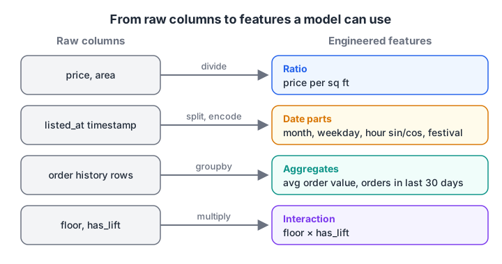
Each engineered feature answers a question a domain expert would ask of the raw columns.

Date and time features

A timestamp like 2026-10-24 19:40 is almost useless to a model as a single number. Broken into parts, it becomes several strong signals: hour of day, day of week, month, weekend flag, and whether it falls in a festival week.

Durations help too. "Days since last purchase" and "account age in months" are often among the most predictive features in churn and fraud models.

import pandas as pd

orders = pd.DataFrame({
    "customer": ["A", "B", "A", "C", "B"],
    "ordered_at": pd.to_datetime(["2026-10-17 13:05", "2026-10-18 21:40",
                                  "2026-10-21 19:55", "2026-10-25 08:15",
                                  "2026-11-02 23:30"]),
})
t = orders["ordered_at"]
orders["hour"] = t.dt.hour
orders["weekday"] = t.dt.day_name()
orders["is_weekend"] = t.dt.day_of_week >= 5
orders["days_since_prev"] = orders.groupby("customer")["ordered_at"].diff().dt.days
print(orders)

days_since_prev is empty for each customer's first order, which is itself informative: new customers behave differently.

Cyclical encoding for hours, days and months

Hour 23 and hour 0 are one hour apart, but as numbers they look 23 apart. A model would treat midnight as the opposite of late evening. The fix is to place the values on a circle with sine and cosine.

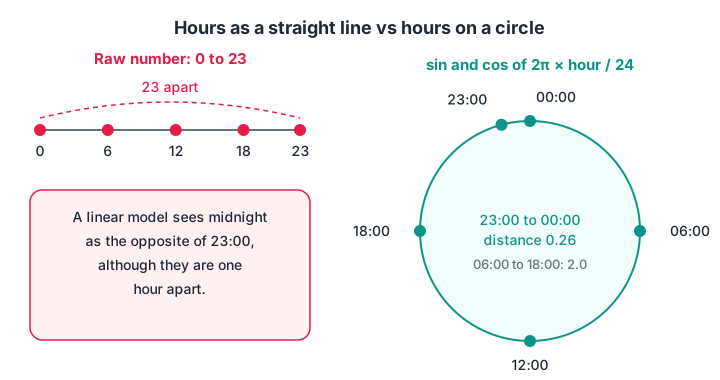
On the circle, 23:00 and 00:00 are neighbours, and 06:00 sits opposite 18:00.

import numpy as np, pandas as pd

hours = pd.Series([0, 6, 12, 18, 23])
hour_sin = np.sin(2 * np.pi * hours / 24)
hour_cos = np.cos(2 * np.pi * hours / 24)
feats = pd.DataFrame({"hour": hours, "sin": hour_sin.round(3), "cos": hour_cos.round(3)})
print(feats)

def gap(a, b):  # distance between two hours in (sin, cos) space
    return np.hypot(feats.sin[a] - feats.sin[b], feats.cos[a] - feats.cos[b]).round(3)
print("\n23:00 vs 00:00:", gap(4, 0), "| 06:00 vs 18:00:", gap(1, 3))

Use the same formula with 7 for weekdays and 12 for months. Tree models cope with raw hours reasonably well, so cyclical encoding matters most for linear models, neural networks and distance-based methods.

Ratios, differences and interactions

Ratios turn two raw numbers into one that carries meaning. Price per square foot, debt-to-income, clicks per visit, and marks per attempt all compare things on a fair basis.

Differences work the same way: "this month's spend minus last month's" captures a trend that neither number shows alone.

Interaction features multiply two columns so a linear model can capture effects that depend on each other. In the broker's case, a high floor adds value only if the building has a lift. The product floor × has_lift lets a linear model learn that.

The block below shows how much one ratio helps a linear model when the true relationship is per-unit.

import numpy as np
from sklearn.linear_model import LinearRegression
from sklearn.model_selection import cross_val_score

rng = np.random.default_rng(4)
n = 500
area = rng.uniform(500, 2500, n)
rate = rng.uniform(3500, 9000, n)            # rupees per sq ft, varies by locality
price = area * rate / 1e5 + rng.normal(0, 3, n)  # lakhs

raw = np.column_stack([area, rate])
engineered = np.column_stack([area, rate, area * rate])   # interaction term

for name, X in [("raw columns", raw), ("with area x rate", engineered)]:
    r2 = cross_val_score(LinearRegression(), X, price, cv=5, scoring="r2").mean()
    print(f"{name:>17}: mean R^2 = {r2:.3f}")

The raw model can only add area and rate together, so it scores well but leaves systematic errors on large, expensive flats. One product column lets the same simple model fit almost perfectly. PolynomialFeatures in scikit-learn can generate every pairwise product automatically, but on wide data that creates hundreds of columns, so add the ones domain knowledge suggests first.

Aggregations and group features

Many datasets have one row per event but you predict per customer, store or device. Group aggregates summarise history into features: a customer's average order value, number of orders in the last 30 days, share of orders cancelled, or how a store's sales compare with the city average.

In pandas, groupby().transform() returns a value for every row, aligned with the original table, which makes it ideal for this.

import pandas as pd

orders = pd.DataFrame({
    "customer": ["A", "A", "A", "B", "B", "C"],
    "amount":   [250, 400, 310, 1200, 900, 150],
    "cancelled": [0, 1, 0, 0, 0, 1],
})
g = orders.groupby("customer")
orders["cust_avg_amount"] = g["amount"].transform("mean").round(1)
orders["cust_orders"] = g["amount"].transform("count")
orders["cust_cancel_rate"] = g["cancelled"].transform("mean").round(2)
orders["vs_own_avg"] = (orders["amount"] / orders["cust_avg_amount"]).round(2)
print(orders.to_string())

vs_own_avg is a favourite in fraud detection. ₹1,200 is normal for customer B and alarming for customer C. The same per-customer summaries drive RFM segmentation in analytics work.

Binning and simple text features

Binning

Binning groups a continuous value into ranges: age into 18–25, 26–35 and so on, or income into quartiles. pd.cut uses fixed edges you choose; pd.qcut makes bins with equal counts.

Binning helps when the effect is a step rather than a slope (a loan rule that changes at age 25), and it makes features easier to explain to business teams. It throws away detail, so don't bin by default.

Text counts

Before reaching for language models, simple counts from text often carry signal: review length, number of exclamation marks, whether a complaint mentions "refund", or the share of capital letters in an SMS. These features are cheap, transparent and quick to test.

How to avoid leakage in feature engineering

A feature is only valid if you could compute it at the moment of prediction. Follow these rules:

1. Use only past data for time-based features. "Orders in the last 30 days" must stop at the prediction date, not include later orders.
2. Never build features from the target. "Average default rate of this customer" includes the label you are predicting.
3. Compute group statistics on training data only, or use cross-fitting as TargetEncoder does.
4. Fit any learned transformation inside a Pipeline, so cross-validation refits it per fold.
5. Check suspiciously strong features. If one feature gives 99% accuracy, it is probably leaking.

Building features that survive these checks takes practice on real business data, which is what a project-led data science programme in Indore gives you time for.

Common feature engineering mistakes

• Creating hundreds of features blindly. More columns mean more noise and slower models; start from domain questions.
• Encoding hour or month as a plain number for linear models. Use sine and cosine.
• Dividing by values that can be zero. Guard ratios with np.where(den > 0, num / den, np.nan).
• Aggregating over the full dataset, future included. That is leakage, even if it feels like summary statistics.
• Keeping features without validating them. Compare cross-validated scores with and without each new feature group.

Key takeaways

• Feature engineering turns raw columns into signals a model can use directly.
• Split timestamps into parts, and encode cyclical parts with sine and cosine.
• Ratios, differences and interactions capture relationships linear models cannot invent.
• Group aggregates summarise history per customer, store or device.
• Every feature must be computable at prediction time from past, non-target data.
• Validate each feature group with cross-validation before keeping it.

Next, the series moves to data ordered in time with time series analysis, where many of these date features return. For quick drills on choosing and validating features, test your feature engineering instincts on Debugshala Test.