Statistics for Data Science: Mean, Spread and Distributions

Suppose you are looking for a rented flat near Bhawarkua for your first job. A broker shows you seven flats with monthly rents of 8,000, 8,500, 9,000, 9,000, 9,500, 10,000 and 45,000 rupees. He says, "Average rent here is about 14,000."

He is not lying. The arithmetic average really is 14,143. But six of the seven flats cost 10,000 or less. The single luxury flat drags the average up and makes the area look more expensive than it is.

That is the whole reason statistics matters in data science: one number can describe data honestly or misleadingly, and you need to know which one to pick.

Why statistics is the base of data science

Map the flat hunt onto the jargon:

• The seven rents are a sample from all flats in the area (the population).
• "Average rent" is a summary statistic, a single number standing in for many.
• The 45,000 flat is an outlier, a value far from the rest.

Statistics is the toolkit for summarising data, measuring uncertainty and deciding whether a pattern is real.

Every later stage of a project, from EDA to model evaluation, uses these tools. If you have not yet seen the bigger picture, what is data science explains where statistics fits among the other skills.

Mean, median and mode: three kinds of "typical"

• Mean: add everything and divide by the count. Sensitive to outliers.
• Median: sort the values and take the middle one. Robust to outliers.
• Mode: the value that appears most often. Useful for categories like "most common plan".

Python's built-in statistics module handles all three, no install needed.

import statistics as st

rents = [8000, 8500, 9000, 9000, 9500, 10000, 45000]

print("Mean:  ", round(st.mean(rents)))
print("Median:", st.median(rents))
print("Mode:  ", st.mode(rents))

without_outlier = rents[:-1]
print("Mean without the 45,000 flat:", round(st.mean(without_outlier)))

The median stays at 9,000 whether or not the luxury flat is included. The mean jumps from about 9,000 to about 14,000. That is why reports on house prices and incomes usually quote the median.

Variance and standard deviation: measuring spread

Two cricket batters both average 40 runs. Batter A scores 38, 41, 39, 42, 40. Batter B scores 0, 95, 5, 90, 10. Same mean, very different reliability.

Variance is the average squared distance from the mean. Standard deviation (SD) is the square root of variance, which brings it back to the original unit (runs, rupees, centimetres).

import numpy as np

a = np.array([38, 41, 39, 42, 40])
b = np.array([0, 95, 5, 90, 10])

for name, runs in [("Batter A", a), ("Batter B", b)]:
    print(f"{name}: mean={runs.mean():.1f}  variance={runs.var(ddof=1):.1f}  SD={runs.std(ddof=1):.1f}")

ddof=1 gives the sample standard deviation, which divides by n − 1 instead of n. Use it when your data is a sample of something larger, which is almost always the case. Note that NumPy's default is ddof=0, while pandas' .std() defaults to ddof=1, so the two can give slightly different answers on the same numbers.

Percentiles and quartiles: where does one value stand?

Your college placement test score is 72. Is that good? It depends on everyone else. A percentile answers that: the 90th percentile is the value below which 90% of scores fall.

The 25th, 50th and 75th percentiles are called quartiles (Q1, median, Q3). The gap between Q1 and Q3 is the interquartile range (IQR), and it gives a common rule for spotting outliers.

import numpy as np

scores = np.array([45, 52, 58, 61, 63, 66, 68, 70, 72, 74, 77, 81, 85, 88, 99])

q1, q2, q3 = np.percentile(scores, [25, 50, 75])
iqr = q3 - q1
print(f"Q1={q1}, median={q2}, Q3={q3}, IQR={iqr}")

my_score = 72
pct = (scores < my_score).mean() * 100
print(f"A score of {my_score} beats {pct:.0f}% of the class")

low, high = q1 - 1.5 * iqr, q3 + 1.5 * iqr
print("Outlier fences:", low, "to", high)
print("Outliers:", scores[(scores < low) | (scores > high)])

None of the scores fall outside the fences here, so there are no outliers by the 1.5 × IQR rule. Try changing 99 to 140 and run it again.

The normal distribution and the 68-95-99.7 rule

Measure the height of 1,000 adults and plot how many fall at each height. You get a bell shape: most people near the middle, fewer at the extremes, roughly symmetric. This shape is the normal distribution.

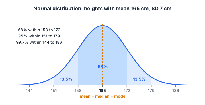
For a normal distribution, about 68% of values fall within 1 SD of the mean, 95% within 2 SD and 99.7% within 3 SD.

The rule makes SD practical. If heights have mean 165 cm and SD 7 cm, you can say about 95% of people are between 151 and 179 cm without seeing the data. You can check this with simulated data:

import numpy as np

rng = np.random.default_rng(42)
heights = rng.normal(loc=165, scale=7, size=10_000)

mean, sd = heights.mean(), heights.std()
for k in (1, 2, 3):
    inside = np.mean(np.abs(heights - mean) <= k * sd) * 100
    print(f"Within {k} SD ({mean - k*sd:.0f} to {mean + k*sd:.0f} cm): {inside:.1f}%")

z = (180 - mean) / sd
print(f"A 180 cm person has z-score {z:.2f}")

A z-score says how many SDs a value sits from the mean. A z-score above 3 or below −3 is rare in normal data and worth a second look.

Correlation vs causation

Correlation measures how strongly two columns move together, on a scale from −1 to +1. Plus one means they rise together perfectly, minus one means one falls as the other rises, and zero means no straight-line relationship.

import numpy as np

hours_studied = np.array([1, 2, 2, 3, 4, 5, 6, 7])
test_marks = np.array([35, 48, 40, 52, 55, 66, 64, 78])
phone_hours = np.array([6, 5, 6, 4, 4, 3, 2, 1])

print("Study hours vs marks:", round(np.corrcoef(hours_studied, test_marks)[0, 1], 2))
print("Phone hours vs marks:", round(np.corrcoef(phone_hours, test_marks)[0, 1], 2))

Both correlations are strong. But does phone use cause lower marks? Maybe. Or maybe students who study more simply have less free time for their phone. The hidden third factor (here, study time) is called a confounder.

A classic example: in Indore, umbrella sales and cases of viral fever both rise in July. Umbrellas do not cause fever. The monsoon drives both. To claim causation you need a controlled experiment, such as an A/B test where you change one thing for a random group and compare.

Common mistakes with statistics

• Quoting the mean for skewed data. Use the median for rents, incomes and delivery times.
• Mixing up sample and population SD. Know whether your tool uses n or n − 1.
• Deleting every outlier. Some outliers are typos, but some are your most important customers. Investigate first.
• Assuming normality. Plot a histogram before using z-scores or the 68-95-99.7 rule.
• Reading causation into correlation. Look for confounders, and test with experiments when the decision matters.

Once these ideas feel natural, the next step is applying them to real tables with NumPy and pandas. Our NumPy arrays tutorial shows how the mean, std and percentile functions work on whole columns at once.

Key takeaways

• The mean is pulled by outliers; the median is not. Report both when in doubt.
• Standard deviation measures spread in the original unit; use ddof=1 for samples.
• Percentiles and the IQR show where a value stands and help flag outliers.
• In a normal distribution, 68%, 95% and 99.7% of values fall within 1, 2 and 3 SD.
• Correlation shows association, not causation. Confounders and experiments matter.