Time Series Analysis in Python: Trend, Seasonality, Forecasts

The owner of a sweet shop near Chappan Dukan has written down his daily sales of kaju katli for two years. Flip through the register and three things jump out.

Sales creep up month after month as the shop gets better known. Every Saturday and Sunday sell more than the weekdays. And in the weeks before Diwali the numbers explode, then fall back.

The owner already "knows" this. Time series analysis turns that feeling into numbers: how fast the growth is, how big the weekend lift is, and how much kaju katli to prepare for next Saturday.

What is time series analysis?

Map the register to the vocabulary:

• Each day's sales, written in order, form a time series.
• The slow month-by-month climb is the trend.
• The weekend bump that repeats every 7 days is seasonality, with a period of 7.
• The day-to-day wobble left over is noise (the residual).
• Guessing next Saturday's sales is forecasting.

Time series analysis is the set of methods for describing, modelling and forecasting data points collected at successive, usually equal, time intervals, where the order of observations carries information.

The order is the whole point. In most datasets you can shuffle the rows without losing anything. Shuffle a time series and you destroy the trend, the seasonality and every relationship between yesterday and today.

This lesson closes the Statistics and EDA series. It uses the date skills from feature engineering and the summary habits from exploratory data analysis. Code targets pandas 2.x and scikit-learn 1.4+; if Python dates are new to you, read Python datetime first.

The components of a time series

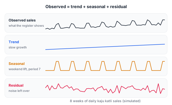
An additive decomposition: observed = trend + seasonal + residual. Each part answers a different business question.

There are two ways the parts can combine:

• Additive: the seasonal swing stays the same size, for example always about 40 extra boxes on weekends.
• Multiplicative: the swing grows with the level, for example weekends always 30% higher. Taking the log of the series turns a multiplicative pattern into an additive one.

A fourth component, the cycle, describes longer rises and falls without a fixed period, such as business cycles. For a few years of shop data you can usually ignore it.

Working with dates in pandas

Everything starts with a DatetimeIndex. Once the index holds real dates, pandas can resample to weeks or months, compute rolling windows and shift values in time.

The block below builds 26 weeks of simulated daily sales with a trend, a weekend lift and noise. Every later block rebuilds the same series so it can run on its own.

import numpy as np, pandas as pd

rng = np.random.default_rng(8)
days = pd.date_range("2026-01-05", periods=182, freq="D")   # starts on a Monday
trend = np.linspace(100, 160, 182)
weekend = np.where(days.day_of_week >= 5, 45, 0)
sales = pd.Series((trend + weekend + rng.normal(0, 8, 182)).round(), index=days)

print(sales.head(8))
print("\nWeekly totals (first 4):")
print(sales.resample("W").sum().head(4))
print("\nAverage by weekday:")
print(sales.groupby(sales.index.day_name()).mean().round(1).sort_values())

resample("W") groups days into weeks, like a groupby on time. The weekday averages expose the seasonality straight away: Saturday and Sunday sit about 45 boxes above the rest.

Trend with rolling averages and decomposition

A rolling mean (moving average) replaces each point with the average of a window around it. A 7-day window averages out the weekly pattern exactly, leaving the trend. Subtract the trend and group what remains by weekday, and you have estimated the seasonal component by hand.

import numpy as np, pandas as pd

rng = np.random.default_rng(8)
days = pd.date_range("2026-01-05", periods=182, freq="D")
sales = pd.Series(np.linspace(100, 160, 182) + np.where(days.day_of_week >= 5, 45, 0)
                  + rng.normal(0, 8, 182), index=days)

trend = sales.rolling(window=7, center=True).mean()
detrended = sales - trend
seasonal = detrended.groupby(detrended.index.day_of_week).transform("mean")
residual = sales - trend - seasonal

print("Trend, first and last full weeks:", trend.dropna().iloc[[0, -1]].round(1).tolist())
print("Seasonal effect Mon..Sun:",
      detrended.groupby(detrended.index.day_of_week).mean().round(1).tolist())
print("Residual std:", round(residual.std(), 2))

The recovered seasonal effects are around −13 for weekdays and +33 for weekends. They sum to about zero, because the trend has absorbed the average level. The residual standard deviation lands close to the 8 we injected as noise.

On your own machine, the statsmodels library does this in one call and adds plots:

from statsmodels.tsa.seasonal import seasonal_decompose  # statsmodels 0.14+
import matplotlib.pyplot as plt

result = seasonal_decompose(sales, model="additive", period=7)
result.plot()
plt.show()

What is autocorrelation?

Autocorrelation is the correlation of a series with a lagged copy of itself. Lag 1 compares each day with the day before; lag 7 compares each day with the same weekday last week.

For the sweet shop, lag-7 autocorrelation is high, because Saturdays look like Saturdays. That tells you a model should use "sales 7 days ago" as a feature. It also tells you that ordinary statistical tests, which assume independent observations, will be misleading on raw time series.

import numpy as np, pandas as pd

rng = np.random.default_rng(8)
days = pd.date_range("2026-01-05", periods=182, freq="D")
sales = pd.Series(np.linspace(100, 160, 182) + np.where(days.day_of_week >= 5, 45, 0)
                  + rng.normal(0, 8, 182), index=days)

for lag in (1, 3, 7, 14):
    print(f"Autocorrelation at lag {lag:>2}: {sales.autocorr(lag=lag):.2f}")

diffed = sales.diff(7).dropna()             # remove weekly pattern and most of the trend
print("\nAfter 7-day differencing, lag 7:", round(diffed.autocorr(lag=7), 2))

After 7-day differencing, the strong positive lag-7 link disappears. It even turns negative, a normal side effect of differencing noisy data, so the weekly pattern no longer dominates.

Stationarity and differencing

A series is stationary when its mean and variance don't drift over time. Classic models such as ARIMA assume stationarity, and our sales clearly aren't: the mean rises.

Differencing fixes this. sales.diff(1) gives the day-to-day change, which removes a steady trend. sales.diff(7) compares each day with the same weekday last week, which removes the weekly pattern too. Formal tests such as the Augmented Dickey-Fuller test (statsmodels.tsa.stattools.adfuller) check stationarity numerically.

How do you evaluate a time series forecast?

You can't use a random train-test split. Random splitting would let the model train on next week to predict this week, which is impossible in real life and makes scores look far better than they are.

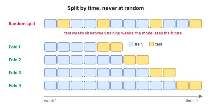
Each fold trains on the past and tests on the period right after it. scikit-learn's TimeSeriesSplit produces exactly these folds.

Follow these steps for any forecast:

1. Sort by time and hold out the most recent period as the test set.
2. Build a naive baseline: tomorrow equals today, or seasonal naive: next Saturday equals last Saturday.
3. Build your model using only information available before each prediction date, such as lag features.
4. Compare both on the same test period with mean absolute error (MAE).
5. Keep the model only if it clearly beats the baseline.

import numpy as np, pandas as pd
from sklearn.linear_model import LinearRegression

rng = np.random.default_rng(8)
days = pd.date_range("2026-01-05", periods=182, freq="D")
sales = pd.Series(np.linspace(100, 160, 182) + np.where(days.day_of_week >= 5, 45, 0)
                  + rng.normal(0, 8, 182), index=days)

df = pd.DataFrame({"y": sales, "lag7": sales.shift(7), "lag14": sales.shift(14),
                   "t": np.arange(182)}).dropna()
train, test = df.iloc[:-28], df.iloc[-28:]             # last 4 weeks held out

naive_mae = (test["y"] - test["lag7"]).abs().mean()     # seasonal naive
model = LinearRegression().fit(train[["lag7", "lag14", "t"]], train["y"])
pred = model.predict(test[["lag7", "lag14", "t"]])
print(f"Seasonal naive MAE: {naive_mae:.1f} boxes")
print(f"Linear model MAE:   {np.abs(test['y'] - pred).mean():.1f} boxes")

The model beats the seasonal naive forecast because it averages two past weeks and adds the trend, so it is less thrown by one noisy week. For full statistical models such as ARIMA and exponential smoothing, statsmodels is the standard Python library; for tree models, these same lag features plug into gradient boosting.

If you would like to build forecasting projects on real sales data with a mentor, Debugshala's Data Science & AI classes, offline or online include a time series module.

Common time series mistakes

• Shuffling before splitting. Always split by time.
• Skipping the naive baseline. Many fancy models lose to "same as last week".
• Using future information in features. A centred rolling mean includes tomorrow; for forecasting, use rolling(...).mean().shift(1).
• Ignoring missing dates. A missing day shifts every lag; use asfreq("D") to expose gaps.
• Forgetting special days. Diwali, Holi and sale events need explicit flags or they ruin the error metric.
• Running standard tests on autocorrelated data. Independence assumptions break, so p-values mislead.

Key takeaways

• A time series is data in time order, and the order carries the information.
• Decompose into trend, seasonality and residual before modelling.
• pandas resample, rolling, shift and diff handle most basic analysis.
• Autocorrelation shows which past lags matter; differencing removes trend and seasonality.
• Split by time, compare against a seasonal naive baseline, and use only past data in features.

That completes the Statistics and EDA series. The next series begins with machine learning foundations, starting from AI vs ML vs deep learning. Before moving on, you can attempt time series and pandas MCQs on Debugshala Test.