

Probability Distributions Explained: Binomial, Poisson, Normal
Binomial, Poisson, normal and exponential distributions explained with PMF, PDF and CDF, a chooser flowchart and Python code that runs without scipy.
Think of the admissions desk at a training institute in Indore. On a normal weekday it gets about 4 phone enquiries an hour. Some hours bring 2 calls, some bring 7, and once in a while an hour passes with none.
The manager wants to know how many people to staff. "Four on average" is not enough. She needs to know how often 8 or more calls arrive at once, because that is when callers hang up.
What she needs is the full picture: the chance of 0 calls, 1 call, 2 calls and so on. That picture is a probability distribution.
What is a probability distribution?
Map the call desk to the terms:
- "Number of calls in one hour" is a random variable: a quantity whose value depends on chance.
- The values it can take (0, 1, 2, 3, …) form its support.
- The table of "value → probability" is its distribution.
A probability distribution is a function that gives the probability of every possible value of a random variable, and all those probabilities add up to 1.
The probability basics tutorial dealt with single events, such as "this order is late". A distribution describes every outcome at once, so it answers any question about the variable: its average, its spread and the chance of extremes.
Discrete vs continuous random variables
The first question to ask about any column is whether it is counted or measured.
| Discrete | Continuous | |
|---|---|---|
| Values | Separate, countable (0, 1, 2, …) | Any value in a range (2.31, 2.317, …) |
| Examples | Calls per hour, defective bulbs in a box, clicks on an ad | Delivery time, height, rainfall in mm |
| Described by | PMF: probability mass function | PDF: probability density function |
| P(exactly one value) | Can be positive, e.g. P(X = 3) = 0.2 | Always 0; use ranges like P(2 < X < 3) |
| Common members | Bernoulli, binomial, Poisson | Uniform, normal, exponential |
The last row surprises many beginners. For a continuous variable, the chance that a delivery takes exactly 30.000000 minutes is zero. You can only ask about intervals, and the probability is the area under the density curve over that interval.
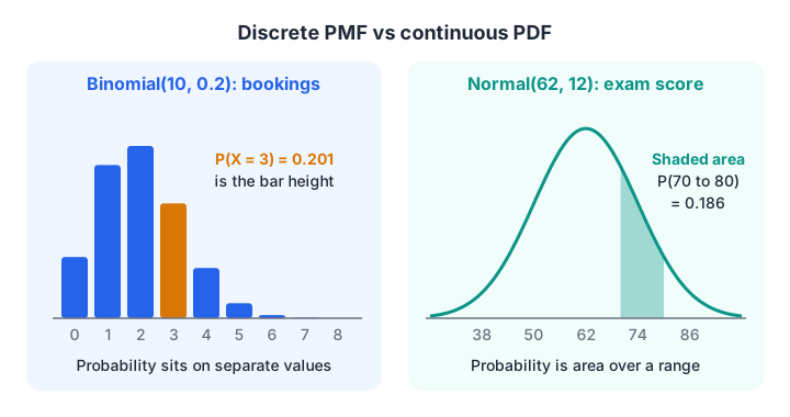
A PMF puts probability on separate bars; a PDF spreads it as area under a curve.
Both kinds share one tool, the CDF (cumulative distribution function). CDF(x) is the probability that the variable is at most x. "What is the chance of 5 or fewer calls?" is a CDF question.
Quick check
For a continuous random variable, what is P(X = 2.5) exactly?
A single point has no width, so it has zero area under the density curve. Only intervals have positive probability.
Discrete distributions: Bernoulli, binomial and Poisson
Bernoulli: one yes-or-no trial
A Bernoulli variable takes the value 1 with probability p and 0 with probability 1 − p. One visitor either signs up for a demo or not. It is the building block for the next two.
Binomial: successes in n trials
Run n independent Bernoulli trials with the same p and count the successes. That count follows a binomial distribution, written Binomial(n, p).
Say 20% of people who call the desk book a demo class. Out of 10 callers today, how many will book? The formula is P(X = k) = C(n, k) × pᵏ × (1 − p)ⁿ⁻ᵏ, where C(n, k) counts the ways to choose which k callers book. Python's math.comb computes C(n, k) directly.
from math import comb

n, p = 10, 0.20
for k in range(0, 7):
    prob = comb(n, k) * p**k * (1 - p)**(n - k)
    print(f"P({k} bookings) = {prob:.3f}  " + "#" * round(prob * 60))

mean = n * p
var = n * p * (1 - p)
print(f"\nMean = {mean}, variance = {var:.2f}")
print(f"P(4 or more) = {1 - sum(comb(n,k)*p**k*(1-p)**(n-k) for k in range(4)):.3f}")
Two bookings is the single most likely result, and four or more bookings happens on roughly 12% of days. Mean n × p and variance n × p × (1 − p) are worth remembering.
Poisson: events in a fixed window
When you count events in a time or space window and there is no fixed number of trials, use the Poisson distribution. It has one parameter, λ (lambda), the average count per window. Calls per hour, website errors per day and potholes per kilometre of road are classic Poisson data.
For the call desk with λ = 4, P(X = k) = e^(−λ) × λᵏ / k!. The manager's question was the chance of 8 or more calls in an hour.
from math import exp, factorial

lam = 4
pmf = [exp(-lam) * lam**k / factorial(k) for k in range(20)]

for k in range(0, 10):
    print(f"P({k} calls) = {pmf[k]:.3f}")

p_8_plus = 1 - sum(pmf[:8])
print(f"\nP(8 or more calls in an hour) = {p_8_plus:.3f}")
print(f"Busy hours in a 9-hour day, on average: {9 * p_8_plus:.2f}")
About 5% of hours bring 8 or more calls. In a 9-hour day, that is roughly one rush hour every two days, a number she can actually plan around.
Quick check
A website gets on average 3 sign-ups per hour, with no fixed number of visitors. Which distribution best models sign-ups per hour?
Events counted in a fixed time window with a known average rate and no fixed number of trials fit a Poisson distribution.
Continuous distributions: uniform, normal and exponential
Uniform
In a uniform distribution every value in a range [a, b] is equally likely. A random number generator's random() is uniform on [0, 1). It is rare in real data but common in simulation and in random search for hyperparameters.
Normal
The normal distribution is the familiar bell curve defined by a mean μ and standard deviation σ. The statistics for data science tutorial covers its shape and the 68-95-99.7 rule, so here we focus on using its CDF.
Python 3.8+ ships statistics.NormalDist, which gives you the PDF, CDF and inverse CDF with no extra install. Suppose exam scores are normal with mean 62 and SD 12.
from statistics import NormalDist

scores = NormalDist(mu=62, sigma=12)

print(f"P(score <= 50)        = {scores.cdf(50):.3f}")
print(f"P(score > 85)         = {1 - scores.cdf(85):.3f}")
print(f"P(70 <= score <= 80)  = {scores.cdf(80) - scores.cdf(70):.3f}")
print(f"Cut-off for top 10%   = {scores.inv_cdf(0.90):.1f}")
inv_cdf answers the reverse question: which score has 90% of students below it? This is how you set a cut-off for a scholarship or flag the top decile of customers.
Exponential: waiting time between events
If calls arrive as a Poisson process with λ = 4 per hour, the waiting time between calls follows an exponential distribution with mean 1/λ = 15 minutes. Its CDF is P(T ≤ t) = 1 − e^(−λt). It is right-skewed: most gaps are short, a few are long.
import numpy as np

lam_per_min = 4 / 60
rng = np.random.default_rng(1)
gaps = rng.exponential(scale=1 / lam_per_min, size=50_000)

print(f"Simulated mean gap: {gaps.mean():.1f} min (theory: {1/lam_per_min:.0f})")
print(f"Simulated P(gap > 30 min): {(gaps > 30).mean():.3f}")
print(f"Formula   P(gap > 30 min): {np.exp(-lam_per_min * 30):.3f}")
The simulation and the formula agree, which is a quick way to check any formula you are unsure of.
How to choose the right distribution
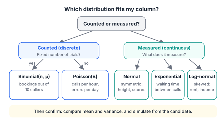
Start with "counted or measured?", then ask what exactly is being counted or measured.
Follow these steps for a new column:
- Decide whether it is counted (discrete) or measured (continuous).
- For counts, ask whether there is a fixed number of trials. Yes points to binomial; no points to Poisson.
- For measurements, plot a histogram. Symmetric and bell-shaped suggests normal; waiting times suggest exponential; long right tails, like income or rent, often fit a log-normal.
- Compare the data's mean and variance with what the candidate distribution predicts.
- Simulate from the fitted distribution and check that the fake data looks like the real data.
To draw the histogram in step 3, you would use matplotlib on your laptop:
import numpy as np
import matplotlib.pyplot as plt

rng = np.random.default_rng(0)
calls = rng.poisson(lam=4, size=1000)

values, counts = np.unique(calls, return_counts=True)
plt.bar(values, counts / counts.sum(), color="#2563eb")
plt.xlabel("Calls per hour")
plt.ylabel("Probability")
plt.title("Simulated Poisson(4) call counts")
plt.show()
The runnable version below does the same checks with numbers instead of a picture, which is also how you would test a column inside a script.
import numpy as np

rng = np.random.default_rng(0)
calls = rng.poisson(lam=4, size=1000)          # pretend this is real data
values, counts = np.unique(calls, return_counts=True)

print("mean =", calls.mean().round(2), " variance =", calls.var(ddof=1).round(2))
for v, c in zip(values, counts):
    print(f"{v:>2} calls: {c / calls.size:.3f}  " + "#" * (c // 10))
Mean and variance both come out close to 4, which is exactly the Poisson signature from the tip above. The next topic, the central limit theorem, explains why the normal distribution keeps appearing even when the raw data is binomial or Poisson.
Common mistakes with distributions
- Assuming everything is normal. Counts, waiting times and money are usually skewed. Check the histogram first.
- Asking for P(X = x) on continuous data. Use a range or the CDF instead.
- Using binomial when trials are not independent. If one caller's decision affects the next, the binomial formula is off.
- Ignoring overdispersion. Count data with variance much bigger than the mean is not Poisson.
- Confusing PDF height with probability. A PDF value can exceed 1; only the area under it is a probability.
Key takeaways
- A distribution gives the probability of every possible value; probabilities add up to 1.
- Discrete variables use a PMF, continuous ones use a PDF, and both have a CDF.
- Binomial counts successes in n fixed trials; Poisson counts events in a window; exponential measures the wait between Poisson events.
math.comb,statistics.NormalDistand numpy's random generator cover these without scipy.- Choose a distribution by the data's story, then confirm with mean, variance and a simulation.
If you would like a mentor to review your distribution-fitting work on real projects, Debugshala's mentor-led Data Science & AI batches include that kind of guided practice. For quick revision, try probability MCQs on Debugshala Test.
FAQ
What are the most important probability distributions for data science?
The normal, binomial, Poisson, uniform and exponential distributions cover most daily work. Bernoulli underlies classification targets, and log-normal is useful for skewed money columns. Learn what story each one tells, its parameters and its mean and variance, rather than memorising formulas.
What is the difference between PMF, PDF and CDF?
A PMF gives the probability of each exact value of a discrete variable. A PDF gives density for a continuous variable, and probability is the area under it. A CDF gives the probability that the variable is at most a given value, and it works for both discrete and continuous variables.
When should I use a binomial distribution instead of Poisson?
Use binomial when there is a fixed number of independent trials, each with the same success probability, such as 50 emails each opened or not. Use Poisson when you count events in a window without a fixed trial count, such as complaints per day. With many trials and a small p, the two give similar answers.
How do I check which distribution my data follows?
Plot a histogram, compare the mean and variance with what each candidate predicts, and simulate from the candidate to see if it looks similar. For a formal check, a Q-Q plot or a goodness-of-fit test helps. In practice, the story behind the data usually narrows the choice to one or two options.
Can I learn probability distributions in a classroom in Indore?
Yes. Debugshala, a training and placement institute at Old Palasia in Indore, covers probability distributions within its Data Science & AI course, both offline and online, in English and Hindi. A free demo class is available before you pay, and graduates from non-IT backgrounds or with a year gap can join.
From the team behind this site
Go further with the Data Science & AI Course at Debugshala
These tutorials are written by Debugshala, a training and placement institute at Old Palasia, Indore. The classroom course adds live mentoring, real projects and interview preparation.
- Offline classes at Old Palasia, Indore
- Free demo class before you pay
- Non-IT, fresher and year-gap friendly
- Placement assistance
700+ students placed · 200+ hiring partners · 4.9★ Google rating
