

Central Limit Theorem Explained with a Python Simulation
See the central limit theorem in action: simulate skewed data in numpy, compute standard error, build confidence intervals and learn when the CLT fails.
Imagine you manage a cloud kitchen in Indore that sells poha, sandwiches and the occasional big party order. Most orders are between Rs 120 and Rs 300, but a few corporate orders run to Rs 4,000. If you plot single order values, you get a lopsided shape with a long tail to the right.
Every evening, your accountant picks 40 orders at random and writes down their average value. After 100 evenings, she has 100 averages. You plot those, expecting the same lopsided shape. Instead you see a neat, symmetric bell.
Nothing about your customers changed. What changed is that you are now looking at averages instead of individual orders. That is the central limit theorem at work.
What is the central limit theorem?
Map the kitchen to the statistics:
- All orders the kitchen will ever take are the population, with some mean μ and standard deviation σ.
- The 40 orders picked each evening are a sample of size n = 40.
- Each evening's average is a sample mean, written x̄.
- The collection of x̄ values across many evenings is the sampling distribution of the mean.
The central limit theorem states that the sampling distribution of the mean approaches a normal distribution with mean μ and standard deviation σ / √n as the sample size n grows, whatever the shape of the population, provided observations are independent and the variance is finite.
Two separate claims hide in that sentence. The shape becomes normal. And the width shrinks with √n. Both matter in practice.
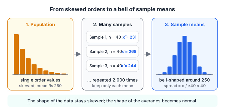
Individual orders are skewed, but the means of repeated samples pile up into a bell around the true mean.
The probability distributions tutorial introduced the exponential distribution, which is strongly right-skewed. It makes a good test case, because if the CLT works there, it works on most real business data.
Quick check
Order values are strongly right-skewed. You take many samples of 100 orders and plot the sample means. What shape do you expect?
The central limit theorem says sample means are approximately normal for large enough n, even when the population is skewed.
Seeing the CLT with a Python simulation
Below, the "population" is 200,000 order values drawn from an exponential distribution with mean Rs 250. Its skewness is about 2, far from the 0 of a normal curve. We then take 2,000 samples of 40 orders each and look at their means.
import numpy as np

rng = np.random.default_rng(42)
population = rng.exponential(scale=250, size=200_000)   # skewed order values

def skew(x):
    return np.mean(((x - x.mean()) / x.std()) ** 3)

means = np.array([rng.choice(population, 40).mean() for _ in range(2000)])

print(f"Population: mean={population.mean():.0f}, SD={population.std():.0f}, skew={skew(population):.2f}")
print(f"Sample means: mean={means.mean():.0f}, SD={means.std():.0f}, skew={skew(means):.2f}")
print(f"Predicted SD of means, sigma/sqrt(n): {population.std() / np.sqrt(40):.0f}")
The mean of the sample means lands right on the population mean. Their spread matches σ / √n closely. And the skewness has dropped from about 2 to roughly 0.3, much closer to symmetric.
If you want to see the bell rather than read the numbers, plot both histograms on your own machine:
import numpy as np
import matplotlib.pyplot as plt

rng = np.random.default_rng(42)
population = rng.exponential(scale=250, size=200_000)
means = [rng.choice(population, 40).mean() for _ in range(2000)]

fig, ax = plt.subplots(1, 2, figsize=(10, 4))
ax[0].hist(population, bins=80, color="#d97706")
ax[0].set_title("Single orders (skewed)")
ax[1].hist(means, bins=40, color="#2563eb")
ax[1].set_title("Means of 40 orders (bell-shaped)")
plt.show()
What is the standard error and why √n matters
The standard deviation of the sample means has its own name: the standard error (SE). It measures how much a sample mean would wobble from one sample to the next.
SE = σ / √n
The square root is the important part. To halve the standard error you need four times as many observations, not twice as many. Going from 40 to 160 orders halves the wobble; going to 640 halves it again.
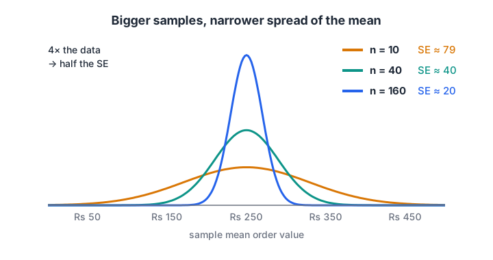
Each fourfold increase in n halves the standard error, so precision gets expensive quickly.
import numpy as np

rng = np.random.default_rng(0)
population = rng.exponential(scale=250, size=200_000)
sigma = population.std()

for n in [10, 40, 160, 640]:
    samples = rng.choice(population, size=(3000, n))
    observed_se = samples.mean(axis=1).std()
    print(f"n={n:>4}: observed SE = {observed_se:6.1f}   formula sigma/sqrt(n) = {sigma/np.sqrt(n):6.1f}")
This is the arithmetic behind every "how many users do we need?" question. When product managers ask why an experiment needs 20,000 users instead of 5,000, the answer is that √n grows slowly.
Quick check
The standard error of a mean is 20 with n = 100. Roughly what will it be with n = 400?
SE = sigma / sqrt(n). Multiplying n by 4 multiplies sqrt(n) by 2, so the SE halves from 20 to 10.
How the CLT powers confidence intervals
Because sample means are approximately normal, you can borrow the normal distribution's properties. About 95% of a normal distribution lies within 1.96 standard deviations of its mean. So an interval of x̄ ± 1.96 × SE captures the true mean in about 95% of samples.
That is a 95% confidence interval. In practice you do not know σ, so you plug in the sample's own standard deviation s. With small samples you would use a t multiplier instead of 1.96, which the hypothesis testing tutorial covers.
The steps for one sample:
- Compute the sample mean x̄ and sample standard deviation s.
- Compute SE = s / √n.
- The interval is x̄ − 1.96 × SE to x̄ + 1.96 × SE.
Does it actually work on skewed data? Repeat the process 2,000 times and count how often the interval contains the true mean.
import numpy as np

rng = np.random.default_rng(3)
true_mean, n, trials = 250, 40, 2000
hits = 0

for _ in range(trials):
    s = rng.exponential(scale=true_mean, size=n)
    se = s.std(ddof=1) / np.sqrt(n)
    low, high = s.mean() - 1.96 * se, s.mean() + 1.96 * se
    hits += low <= true_mean <= high

print(f"One example interval: Rs {low:.0f} to Rs {high:.0f}")
print(f"Coverage: {hits / trials:.1%} of intervals contained the true mean (target 95%)")
Coverage comes out a little under 95%, around 93%. That gap is honest: with skewed data and n = 40, the normal approximation is good but not perfect. Raise n to 200 and the coverage moves closer to 95%.
When the central limit theorem breaks down
The CLT has conditions, and real data sometimes violates them.
| Condition | What goes wrong if it fails | Example |
|---|---|---|
| Independent observations | SE is underestimated, intervals too narrow | Several orders from the same office on the same day |
| Finite variance | Means never settle into a bell | Extremely heavy-tailed data such as a Cauchy distribution |
| Large enough n | Sampling distribution still skewed | n = 10 from very skewed revenue data |
| Random sampling | Mean is biased, CLT cannot fix it | Only sampling weekday lunch orders |
The finite-variance case is easy to demonstrate. A Cauchy distribution has such heavy tails that its variance is undefined. Averages of Cauchy samples never calm down, no matter how large n gets.
import numpy as np

rng = np.random.default_rng(5)
for n in [10, 100, 1_000, 10_000]:
    exp_means = rng.exponential(1.0, size=(500, n)).mean(axis=1)
    cauchy_means = rng.standard_cauchy(size=(500, n)).mean(axis=1)
    print(f"n={n:>6}: range of exponential means={np.ptp(exp_means):6.2f}   "
          f"range of Cauchy means={np.ptp(cauchy_means):9.1f}")
Both use scale 1, so the ranges are comparable. The exponential means tighten as n grows. The Cauchy means stay wild. Real data with a handful of enormous values, like viral social posts or whale customers in a game, can behave closer to the Cauchy case than you would like.
The last row of the table matters most. The CLT describes how a random sample behaves. If your sample is biased, it will happily give you a precise, bell-shaped estimate of the wrong number. Sampling techniques explains how to avoid that.
Common mistakes with the central limit theorem
- Thinking the CLT makes the data normal. It makes the sample mean approximately normal. Individual orders stay skewed.
- Treating n ≥ 30 as a law. It is a rule of thumb for mildly skewed data. Revenue or claim amounts may need hundreds.
- Ignoring dependence. Repeated measurements of the same user are not independent; group them or use methods built for clustered data.
- Using the CLT to excuse a biased sample. Precision is not accuracy.
- Forgetting it applies to sums and proportions too. A conversion rate is a mean of 0s and 1s, so the CLT covers it. That is why A/B testing can compare conversion rates with normal-based tests.
The CLT, standard error and confidence intervals form a single chain of reasoning that every data science interview probes. Debugshala's hands-on data science programme works through simulations like these in class, and you can test your statistics basics with free quizzes on Debugshala Test.
Key takeaways
- The CLT is about sample means, not raw data: their distribution becomes normal as n grows.
- The mean of the sample means equals the population mean, and their spread is the standard error σ / √n.
- Four times the data gives half the uncertainty.
- The CLT is why x̄ ± 1.96 × SE works as a 95% confidence interval on skewed business data.
- It needs independence, finite variance, a big enough n and a random sample.
Next in the series, Bayes' theorem shows how to update a probability when new evidence arrives.
FAQ
Why is the central limit theorem important in data science?
It lets you use normal-distribution tools on data that is not normal. Confidence intervals, z-tests, t-tests and most A/B testing calculators all rely on the sample mean being approximately normal. Without the CLT, you would need a different method for every shape of data.
What sample size is enough for the central limit theorem?
There is no single number. For roughly symmetric data, 20 to 30 observations are usually enough. For skewed data such as revenue, you may need 100 or more. The safest approach is to simulate: resample your own data and check whether the sample means look normal.
Does the central limit theorem apply to proportions?
Yes. A proportion, such as a click-through rate, is the mean of a column of 0s and 1s. The CLT says it is approximately normal with standard error √(p(1 − p) / n). The approximation is good when both n × p and n × (1 − p) are at least about 10.
What is the difference between standard deviation and standard error?
Standard deviation describes how spread out individual values are. Standard error describes how much a sample mean would vary from sample to sample. Standard error equals the standard deviation divided by √n, so it shrinks as you collect more data while the standard deviation does not.
Where can I learn statistics like the CLT in Indore?
Debugshala, a training and placement institute at Old Palasia in Indore, teaches the central limit theorem and inference within its Data Science & AI course. Classes run offline and online in English and Hindi, a free demo class is offered before you pay, and freshers from non-IT backgrounds can join.
From the team behind this site
Go further with the Data Science & AI Course at Debugshala
These tutorials are written by Debugshala, a training and placement institute at Old Palasia, Indore. The classroom course adds live mentoring, real projects and interview preparation.
- Offline classes at Old Palasia, Indore
- Free demo class before you pay
- Non-IT, fresher and year-gap friendly
- Placement assistance
700+ students placed · 200+ hiring partners · 4.9★ Google rating
