Probability for Data Science: Rules and Python Examples

Picture a food delivery app working in Indore. Last month it delivered 2,000 orders in Vijay Nagar, and 140 of them arrived late. A new customer opens the app tonight and asks a simple question: "Will my biryani be late?"

Nobody can promise yes or no. What you can say is that about 7 in 100 orders were late, so the chance is roughly 0.07. That number is a probability.

Now add a detail. Of the 600 orders placed during rain, 90 were late. Suddenly the chance for a rainy evening is 0.15, more than double. Updating a probability when you learn something new is the everyday work of data science.

What is probability in data science?

Map the delivery story to the vocabulary:

• Placing one order and seeing what happens is an experiment (statisticians also call it a trial).
• "On time" and "late" together form the sample space, the list of every possible outcome.
• "Late" is an event, a set of outcomes you care about.
• 140 out of 2,000 is the empirical probability of that event.

Probability is a number from 0 (impossible) to 1 (certain) that measures how likely an event is, calculated as favourable outcomes divided by all equally likely outcomes, or estimated from observed frequencies.

The classical way counts outcomes: a fair die has six faces, so P(rolling a 4) = 1/6. The empirical way counts history: 140 late orders out of 2,000 gives 0.07. Real projects mostly use the empirical way, because nobody hands you the true probability of a customer churning.

If you are still settling into Python, the Python operators tutorial covers the division and comparison operators used below.

import numpy as np

# Classical probability: count outcomes
faces = [1, 2, 3, 4, 5, 6]
p_even = sum(1 for f in faces if f % 2 == 0) / len(faces)
print("P(even) on a fair die:", p_even)

# Empirical probability: count history
late = np.array([1] * 140 + [0] * 1860)   # 1 = late, 0 = on time
print("Orders:", late.size, "| late:", late.sum())
print("P(late) =", late.mean())

Notice the trick in the last line. When late orders are stored as 1 and on-time orders as 0, the mean of the column is the probability. You will use this shortcut constantly in pandas.

The complement and addition rules

The complement rule

P(not A) = 1 − P(A). If 7% of orders are late, 93% are on time. This turns "at least one" questions into easy ones: the chance that five orders are all on time is 0.93⁵, about 0.70, so the chance of at least one late order is about 0.30.

The addition rule

For two events A and B, P(A or B) = P(A) + P(B) − P(A and B). You subtract the overlap because adding P(A) and P(B) counts the shared part twice.

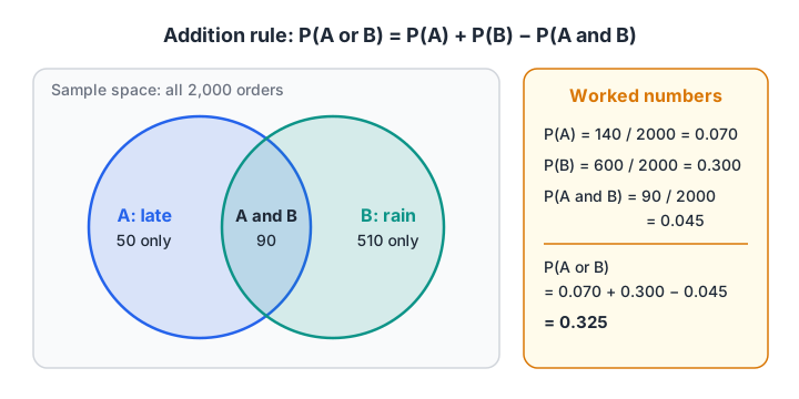
The overlap (A and B) is counted twice when you add P(A) and P(B), so the addition rule subtracts it once.

If two events can never happen together, they are mutually exclusive and the overlap is zero. "Order is late" and "order is on time" are mutually exclusive. "Order is late" and "order was placed in rain" are not.

import pandas as pd

orders = pd.DataFrame({
    "late": [1]*90 + [0]*510 + [1]*50 + [0]*1350,
    "rain": [1]*600 + [0]*1400,
})
p_late = orders["late"].mean()
p_rain = orders["rain"].mean()
p_both = ((orders["late"] == 1) & (orders["rain"] == 1)).mean()

print(f"P(late)          = {p_late:.3f}")
print(f"P(rain)          = {p_rain:.3f}")
print(f"P(late and rain) = {p_both:.3f}")
print(f"P(late or rain)  = {p_late + p_rain - p_both:.3f}")
print("Check by counting:", ((orders.late == 1) | (orders.rain == 1)).mean())

What is conditional probability?

Conditional probability answers "how likely is A, given that B already happened?" It is written P(A | B) and read "probability of A given B". The formula is P(A | B) = P(A and B) / P(B).

The idea is easier than the formula. Once you know it is raining, you ignore every dry-weather order and look only at the 600 rainy ones. Of those, 90 were late, so P(late | rain) = 90 / 600 = 0.15.

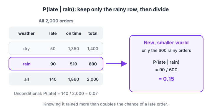
Conditioning on rain means ignoring the dry row and dividing by the rainy total only.

pandas does this for you with crosstab and normalize="index", which divides each row by its own total.

import pandas as pd

orders = pd.DataFrame({
    "weather": ["rain"]*600 + ["dry"]*1400,
    "status":  ["late"]*90 + ["on time"]*510 + ["late"]*50 + ["on time"]*1350,
})

counts = pd.crosstab(orders["weather"], orders["status"], margins=True)
print(counts, "\n")

# Each row now sums to 1: P(status | weather)
print(pd.crosstab(orders["weather"], orders["status"], normalize="index").round(3))

The output shows P(late | dry) is about 0.036 and P(late | rain) is 0.15. A model that predicts delays would treat weather as a strong feature for exactly this reason.

Independent events and the multiplication rule

Two events are independent when knowing one tells you nothing about the other. Formally, A and B are independent when P(A | B) = P(A), which is the same as P(A and B) = P(A) × P(B).

The multiplication rule in general form is P(A and B) = P(A) × P(B | A). When the events are independent, P(B | A) is just P(B), and you can multiply the plain probabilities.

In the delivery data, P(late) is 0.07 but P(late | rain) is 0.15, so lateness and rain are dependent.

import pandas as pd

orders = pd.DataFrame({
    "late": [1]*90 + [0]*510 + [1]*50 + [0]*1350,
    "rain": [1]*600 + [0]*1400,
})
p_late, p_rain = orders.late.mean(), orders.rain.mean()
p_both = (orders.late & orders.rain).mean()

print("P(late) x P(rain) =", round(p_late * p_rain, 4))
print("P(late and rain)  =", round(p_both, 4))
print("Independent?", abs(p_both - p_late * p_rain) < 0.005)

Some models assume independence on purpose. The Naive Bayes classifier treats every word in an email as independent of the others, and still works well.

Expected value: putting probability to work

The expected value of a random outcome is the sum of each outcome multiplied by its probability: the average result per attempt over many repeats.

Say the app offers Rs 50 cashback on every late order. With P(late) = 0.07, the expected cost per order is 0.07 × 50 = Rs 3.50. On 2,000 orders a month that is about Rs 7,000, which finance can plan for.

outcomes = {"on time": 0, "late": 50}      # cashback paid in rupees
probs    = {"on time": 0.93, "late": 0.07}

ev = sum(outcomes[k] * probs[k] for k in outcomes)
print(f"Expected cashback per order: Rs {ev:.2f}")
print(f"Expected cost for 2,000 orders: Rs {ev * 2000:,.0f}")

# Rainy evenings are riskier
ev_rain = 0.15 * 50
print(f"Expected cashback per rainy order: Rs {ev_rain:.2f}")

The law of large numbers: why data beats guesses

You might wonder why 140 out of 2,000 is trusted as "the" probability. The law of large numbers says that as you repeat an experiment more times, the observed frequency settles closer to the true probability.

With 10 orders you could easily see 0 or 3 late ones, giving 0% or 30%. With 10,000 orders the estimate sits very close to 7%.

import numpy as np

rng = np.random.default_rng(7)
true_p = 0.07

for n in [10, 100, 1_000, 10_000, 100_000]:
    sample = rng.random(n) < true_p      # True means late
    print(f"n = {n:>7,}: estimated P(late) = {sample.mean():.4f}")

So a new restaurant with 12 orders and zero late deliveries has proven nothing yet. The central limit theorem later tells you exactly how wide that uncertainty is.

Common mistakes with probability

• Adding probabilities of overlapping events. P(A or B) is not P(A) + P(B) unless the events cannot happen together. Subtract the overlap.
• Multiplying dependent events as if they were independent. Rain and late deliveries move together, so P(late) × P(rain) underestimates how often both happen.
• Swapping the condition. P(late | rain) and P(rain | late) answer different questions. Mixing them up is the classic error behind misleading headlines.
• Trusting tiny samples. A probability from 15 rows can be far from the truth.
• The gambler's fallacy. If five orders in a row were on time, the next one is not "due" to be late. Independent trials have no memory.

Probability questions appear in most aptitude rounds. You can solve probability and aptitude MCQs on Debugshala Test and then confirm your answers with the simulations above.

Quick check

Key takeaways

• Probability runs from 0 to 1. In data science you mostly estimate it as favourable rows divided by total rows, or the .mean() of a 0/1 column.
• Use the complement rule for "at least one" questions and subtract the overlap in the addition rule.
• Conditional probability shrinks the world to the rows where the condition holds. pd.crosstab(..., normalize="index") computes it in one line.
• Independence means P(A and B) = P(A) × P(B). Check it in data before assuming it.
• The law of large numbers is why bigger samples give more trustworthy probabilities.

Next in this series, probability distributions describe the full pattern of outcomes, not just one event. If you prefer to learn these ideas with a mentor and weekly practice, a statistics-heavy data science course in Indore can give you that structure.