

Outlier Detection Methods: Z-Score, IQR, MAD and Mahalanobis
Outlier detection explained with electricity bills: z-score masking, the IQR rule, modified z-score, Mahalanobis distance and what to do with each outlier.
The secretary of a housing society in Vijay Nagar collects the monthly electricity bills of 200 flats. Most fall between ₹1,500 and ₹3,500. Two stand out: one flat shows ₹48,000 and another shows ₹9,200.
A phone call settles both. The ₹48,000 bill was a meter misread; the real figure was ₹4,800. The ₹9,200 bill is genuine: that family runs three air conditioners and a home bakery.
Both were outliers. One was an error to fix, the other a real customer the electricity board would very much like to understand. Outlier detection finds both; only you can tell them apart.
What is an outlier in data science?
Map the bills to the language:
- The 200 bills are your distribution.
- The ₹48,000 bill is an error outlier, caused by measurement or entry mistakes.
- The ₹9,200 bill is a genuine outlier, a true but rare value.
- The rule that flagged them is an outlier detection method.
Outlier detection is the process of identifying observations that deviate strongly from the pattern of the rest of the data, using statistical rules or models, so they can be investigated and handled deliberately.
Outliers matter because many statistics are fragile. One ₹48,000 bill lifts the society's mean bill by over ₹200, and a regression line can tilt towards a single extreme point. Medians, percentiles and tree models are far less affected.
You will usually spot candidates first in the exploratory data analysis stage, often after dealing with missing data. This article targets Python 3.12+, numpy and scikit-learn 1.4+.
Three kinds of outliers
- Global (point) outliers: extreme compared with everything, like the ₹48,000 bill.
- Contextual outliers: normal in general but odd in context. ₹3,000 is an ordinary bill in May but strange for a flat that was locked all month.
- Collective outliers: a group of values that is unusual together, such as five days of zero sales at a shop that never closes.
This article focuses on point outliers in tabular data. Detecting unusual events in streams and logs is covered under anomaly detection.
The z-score method and its weakness
A z-score tells you how many standard deviations a value is from the mean: z = (x − mean) / std. A common rule flags any point with |z| > 3. For roughly normal data, fewer than 0.3% of points pass that threshold by chance, as the normal distribution predicts.
The catch is that the mean and standard deviation are themselves pulled by outliers. A huge value inflates the standard deviation, which shrinks every z-score, including its own. This is called masking: big outliers hide themselves and their neighbours.
import numpy as np

rng = np.random.default_rng(11)
bills = rng.normal(2500, 450, 198).round()
bills = np.append(bills, [48000, 9200])      # misread meter, genuine big user

z = (bills - bills.mean()) / bills.std()
print("Mean bill:", round(bills.mean()), "| std:", round(bills.std()))
print("z of ₹48,000:", round(z[-2], 1), "| z of ₹9,200:", round(z[-1], 1))
print("Flagged with |z| > 3:", bills[np.abs(z) > 3])
The ₹48,000 bill inflates the standard deviation so much that the ₹9,200 bill gets a z-score well under 3 and escapes. Remove the ₹48,000 error and the ₹9,200 bill jumps to a z-score above 10.
Quick check
Why can one very large value hide other outliers when you use z-scores?
The z-score divides by the standard deviation, which a huge value inflates. This masking effect does not affect percentile-based rules much.
The IQR rule (Tukey's fences)
The interquartile range (IQR) is the distance between the 25th percentile (Q1) and the 75th percentile (Q3), the middle half of the data. John Tukey's rule flags anything below Q1 − 1.5×IQR or above Q3 + 1.5×IQR. Using 3×IQR instead marks only "far out" points.
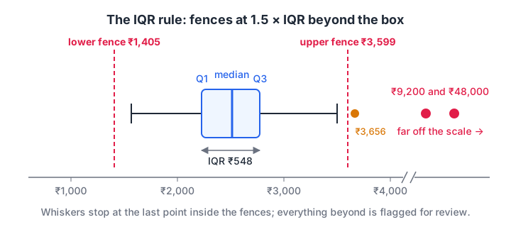
Points beyond the fences are flagged. The fences depend on percentiles, so one huge value cannot move them much.
Because percentiles barely move when you add one extreme value, the IQR rule resists masking. It is also exactly what a box plot's whiskers show, so your chart and your rule agree.
import numpy as np

rng = np.random.default_rng(11)
bills = np.append(rng.normal(2500, 450, 198).round(), [48000, 9200])

q1, q3 = np.percentile(bills, [25, 75])
iqr = q3 - q1
low, high = q1 - 1.5 * iqr, q3 + 1.5 * iqr
print(f"Q1={q1:.0f}  Q3={q3:.0f}  IQR={iqr:.0f}")
print(f"Fences: below {low:.0f} or above {high:.0f}")
print("Flagged:", np.sort(bills[(bills < low) | (bills > high)]))
Both real problems are flagged now. With 198 normal-ish values, the 1.5×IQR rule may also flag one or two ordinary bills near the edges. That is expected: about 0.7% of normally distributed data falls outside the fences.
Quick check
Q1 is 40 and Q3 is 60. Using the 1.5×IQR rule, which value is flagged?
IQR = 20, so the upper fence is 60 + 30 = 90. Only 95 lies above it.
The modified z-score (median absolute deviation)
The modified z-score swaps the mean for the median and the standard deviation for the median absolute deviation (MAD): the median of |x − median|. Iglewicz and Hoaglin suggested the formula 0.6745 × (x − median) / MAD and a cut-off of 3.5.
It reads like a z-score but is as robust as the IQR rule.
import numpy as np

rng = np.random.default_rng(11)
bills = np.append(rng.normal(2500, 450, 198).round(), [48000, 9200])

median = np.median(bills)
mad = np.median(np.abs(bills - median))
modified_z = 0.6745 * (bills - median) / mad
print("Median:", median, "| MAD:", mad)
print("Modified z of the last two:", modified_z[-2:].round(1))
print("Flagged (> 3.5):", bills[np.abs(modified_z) > 3.5])
Which univariate method should you use?
| Method | Centre and spread | Robust to masking? | Best for |
|---|---|---|---|
| z-score, |z| > 3 | Mean and standard deviation | No | Clean, roughly normal data |
| IQR rule, 1.5×IQR | Quartiles | Yes | Skewed data, matches box plots |
| Modified z, > 3.5 | Median and MAD | Yes | Robust scores you can rank |
For skewed columns such as incomes or bills, try a log transform first. Many "outliers" on the raw scale are ordinary on the log scale.
How do you detect multivariate outliers?
Some points are only odd in combination. A flat with a ₹1,200 bill is normal. A flat with 4 bedrooms is normal. A 4-bedroom flat with a ₹1,200 bill in May is strange and worth a check for meter tampering.
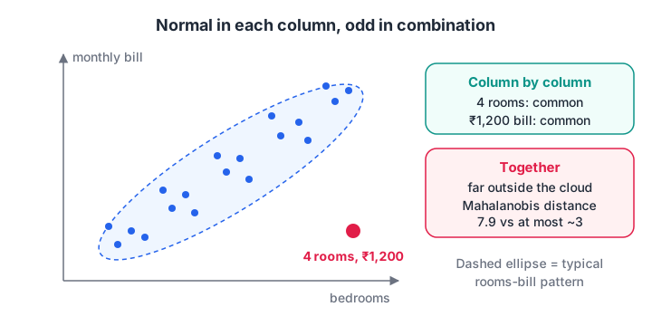
The rose point passes every single-column test but sits far from the cloud, which Mahalanobis distance catches.
Mahalanobis distance measures how far a point is from the centre of the data, accounting for the correlation between columns. It uses the inverse of the covariance matrix, the same idea from linear algebra for data science.
import numpy as np

rng = np.random.default_rng(2)
rooms = rng.integers(1, 5, 300).astype(float)
bill = 900 + 650 * rooms + rng.normal(0, 250, 300)
X = np.column_stack([np.append(rooms, 4), np.append(bill, 1200)])  # odd flat last

centre = X.mean(axis=0)
inv_cov = np.linalg.inv(np.cov(X, rowvar=False))
diff = X - centre
d2 = np.einsum("ij,jk,ik->i", diff, inv_cov, diff)   # squared Mahalanobis
print("Bill z-score of the odd flat:", round((1200 - bill.mean()) / bill.std(), 2))
print("Mahalanobis distance of the odd flat:", round(np.sqrt(d2[-1]), 2))
print("Top 3 distances:", np.sort(np.sqrt(d2))[-3:].round(2))
Its bill alone is under two standard deviations below average, yet its Mahalanobis distance is far above every other flat. For data with many columns or curved patterns, scikit-learn's IsolationForest and LocalOutlierFactor do the same job without assuming a normal shape. Isolation Forest flags points that are easy to separate with a few random splits; anomaly detection walks through both.
What should you do with outliers?
Follow these steps for every flagged point:
- Investigate. Look at the full row. Is it physically possible? Does a source document disagree?
- Fix errors. Correct typos when you can (₹48,000 back to ₹4,800).
- Remove only true errors you cannot fix. Record how many and why.
- Cap genuine extremes if a model is sensitive. Winsorising replaces values beyond, say, the 1st and 99th percentiles with those percentiles.
- Transform skewed columns. A log or square-root transform pulls in the long tail.
- Or keep them and use robust tools. Median-based statistics,
RobustScaler, Huber regression and tree models tolerate extremes well.
For fraud, equipment failure or rare diseases, the outliers are the signal. Deleting them would delete the thing you were hired to find.
Learning to argue which points to keep is a skill best built on real messy data, and the Indore data science batch at Debugshala practises it on project datasets.
Common mistakes in outlier detection
- Deleting every flagged point. Detection is a prompt to look, not a verdict.
- Using z-scores on heavily skewed data. The rule assumes a roughly normal shape.
- Removing outliers from the test set. Real users will send extreme values; your evaluation should include them.
- Detecting on the full dataset before splitting. Thresholds should be learned from training data.
- Checking columns one at a time only. Combination outliers slip through.
Key takeaways
- Outliers can be errors or genuine rare values; detection flags, investigation decides.
- The z-score rule is simple but suffers from masking.
- The IQR rule and the modified z-score (MAD) are robust and work better on real, skewed data.
- Use Mahalanobis distance or Isolation Forest for outliers that only appear in combination.
- Fix, remove, cap, transform or keep, and record the choice for each case.
Outliers also affect how you rescale columns, which is the next step: scaling and encoding in data preprocessing. For practice spotting fences and z-scores quickly, try outlier and statistics questions on Debugshala Test.
FAQ
What is the best method to detect outliers?
For a single numeric column, the IQR rule or the modified z-score is the safest default because both resist masking. Use the plain z-score only on clean, roughly normal data. For several columns at once, use Mahalanobis distance on roughly normal data or Isolation Forest for anything more complex.
Should I always remove outliers?
No. Remove only values you have confirmed as errors and cannot correct. Genuine extremes often carry important information, such as fraud or rare high-value customers. When they distort a sensitive model, prefer capping, a log transform or a robust method over deletion, and record what you changed.
What is the 1.5 IQR rule?
The 1.5 IQR rule flags any value below Q1 minus 1.5 times the interquartile range, or above Q3 plus 1.5 times it. The interquartile range is Q3 minus Q1. It was proposed by John Tukey and matches the whiskers on a standard box plot.
What is the difference between an outlier and an anomaly?
The terms overlap. "Outlier" usually means an extreme value in a static dataset, found with statistical rules during analysis. "Anomaly" is common in monitoring and fraud, where the goal is to flag unusual events as they happen, often with machine learning models. The methods are closely related.
Is outlier detection taught in Debugshala's data science course in Indore?
Yes. Outlier detection, robust statistics and preprocessing are part of Debugshala's Data Science & AI course, offered at the Old Palasia campus in Indore and online. Classes run in English and Hindi, with a free demo class before you pay. Fresh graduates and career switchers are welcome.
From the team behind this site
Go further with the Data Science & AI Course at Debugshala
These tutorials are written by Debugshala, a training and placement institute at Old Palasia, Indore. The classroom course adds live mentoring, real projects and interview preparation.
- Offline classes at Old Palasia, Indore
- Free demo class before you pay
- Non-IT, fresher and year-gap friendly
- Placement assistance
700+ students placed · 200+ hiring partners · 4.9★ Google rating
