

Exploratory Data Analysis (EDA) in Python: A 7-Step Guide
Exploratory data analysis step by step in pandas: structure, quality checks, univariate and bivariate analysis, segments and written findings, with code.
Suppose a friend in Indore asks you to price his 2017 hatchback. You open a used-car website and scroll through 300 listings. Without planning to, you start noticing things: diesel cars cost more, cars past 1,00,000 km drop sharply, a few listings say ₹1 because the seller typed it wrong.
Ten minutes of scrolling gave you a feel for the market, a list of suspicious entries and a guess about what drives the price. Nobody built a model yet.
That scrolling, done carefully and with code, is exploratory data analysis. The listings are your dataset, "what drives price" is your question, the ₹1 cars are data quality problems and your guesses are hypotheses.
What is exploratory data analysis?
Exploratory data analysis (EDA) is the process of summarising and visualising a dataset to understand its structure, spot errors and patterns, and form hypotheses before building any model.
The statistician John Tukey popularised the term in the 1970s. His point still holds: look at the data before you trust any method on it. A model trained on the ₹1 listings would learn nonsense, and no accuracy metric would tell you why.
EDA sits right after data collection in the data science lifecycle. It feeds every later step: what to clean, which features to build, which model family suits the problem.
This guide uses pandas 2.x on Python 3.12+. If DataFrames are new to you, start with the pandas DataFrame tutorial.
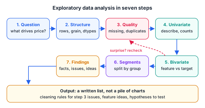
EDA is a loop: a surprise in step 5 often sends you back to check quality or reframe the question.
A sample dataset to explore
Every block below builds the same small dataset of 400 used-car listings, so each one runs on its own. The numbers are simulated but follow realistic patterns, plus a few planted mistakes.
import numpy as np, pandas as pd

rng = np.random.default_rng(42)
n = 400
year = rng.integers(2010, 2024, n)
km = (2025 - year) * rng.normal(11000, 3000, n).clip(3000)
fuel = rng.choice(["Petrol", "Diesel", "CNG"], n, p=[0.55, 0.35, 0.10])
price = 9 * 0.88 ** (2025 - year) * np.where(fuel == "Diesel", 1.2, 1.0) * (1 - km / 900000) * rng.normal(1, 0.08, n)
df = pd.DataFrame({"year": year, "km": km.round(), "fuel": fuel,
                   "owners": rng.choice([1, 2, 3], n, p=[0.6, 0.3, 0.1]),
                   "price_lakh": price.round(2)})
df.loc[[5, 77], "price_lakh"] = 0.0001          # typing errors
df.loc[rng.choice(n, 25, replace=False), "km"] = np.nan

print(df.shape)
print(df.head())
print(df.dtypes)
Steps 1 to 3: question, structure and quality
Step 1: frame the question
Write one sentence: "Which factors explain the asking price of a used car?" It decides which column is the target (price) and which are candidate features. Without a question, EDA turns into making every possible chart.
Step 2: check the structure
Find the grain of the data: what does one row represent? Here it is one listing. Then check the number of rows, the column types and whether numbers were read as text. A price column stored as strings ("4,50,000") will silently break every summary.
Step 3: check data quality
Count missing values, duplicates and impossible values. You are not fixing them yet. You are noting them, because how you fix them depends on why they happened. Handling missing data covers that decision in depth.
import numpy as np, pandas as pd

rng = np.random.default_rng(42)
n = 400
year = rng.integers(2010, 2024, n)
km = (2025 - year) * rng.normal(11000, 3000, n).clip(3000)
fuel = rng.choice(["Petrol", "Diesel", "CNG"], n, p=[0.55, 0.35, 0.10])
price = 9 * 0.88 ** (2025 - year) * np.where(fuel == "Diesel", 1.2, 1.0) * (1 - km / 900000) * rng.normal(1, 0.08, n)
df = pd.DataFrame({"year": year, "km": km.round(), "fuel": fuel, "price_lakh": price.round(2)})
df.loc[[5, 77], "price_lakh"] = 0.0001
df.loc[rng.choice(n, 25, replace=False), "km"] = np.nan

print("Missing per column:\n", df.isna().sum(), sep="")
print("\nDuplicate rows:", df.duplicated().sum())
print("\nPrices below 0.1 lakh (suspicious):")
print(df[df["price_lakh"] < 0.1])
Step 4: univariate analysis, one column at a time
Univariate analysis describes each column alone. For numeric columns, look at the centre, the spread, the range and the shape. For categories, look at the counts.
describe() is the workhorse. Read its output like a checklist:
- Is the minimum or maximum impossible? A price of 0.0001 lakh is ₹10.
- Is the mean far from the median (the 50% row)? That signals skew.
- Is the standard deviation zero? Then the column is constant and useless.
For categorical columns, value_counts(normalize=True) shows the share of each level. Rare levels, with only a handful of rows, will matter later when you encode categories.
import numpy as np, pandas as pd

rng = np.random.default_rng(42)
n = 400
year = rng.integers(2010, 2024, n)
km = (2025 - year) * rng.normal(11000, 3000, n).clip(3000)
fuel = rng.choice(["Petrol", "Diesel", "CNG"], n, p=[0.55, 0.35, 0.10])
price = 9 * 0.88 ** (2025 - year) * np.where(fuel == "Diesel", 1.2, 1.0) * (1 - km / 900000) * rng.normal(1, 0.08, n)
df = pd.DataFrame({"year": year, "km": km.round(), "fuel": fuel, "price_lakh": price.round(2)})

print(df[["km", "price_lakh"]].describe().round(2))
print("\nSkewness:\n", df[["km", "price_lakh"]].skew().round(2), sep="")
print("\nFuel share:\n", df["fuel"].value_counts(normalize=True).round(2), sep="")
A positive skew for price means a long tail of expensive cars. That tail is normal for prices and incomes, and it hints that a log transform may help a linear model later.
Quick check
The mean of a price column is 6.8 lakh and the median is 4.1 lakh. What does this suggest?
A mean well above the median is pulled up by a long tail of large values, which is right skew.
Step 5: bivariate analysis, how columns relate
Bivariate analysis looks at two columns together, usually a feature against the target. The right tool depends on the column types.
| Pair of types | Numbers to compute | Plot to draw |
|---|---|---|
| Numeric vs numeric | Correlation (Pearson or Spearman) | Scatter plot |
| Category vs numeric | groupby().agg(["mean", "median", "count"]) |
Box plot per category |
| Category vs category | pd.crosstab(..., normalize="index") |
Stacked or grouped bar |
| Time vs numeric | Resampled mean or sum | Line chart |
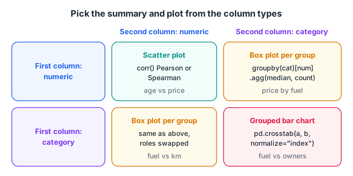
Pick the summary and the plot from the types of the two columns, not from habit.
import numpy as np, pandas as pd

rng = np.random.default_rng(42)
n = 400
year = rng.integers(2010, 2024, n)
km = (2025 - year) * rng.normal(11000, 3000, n).clip(3000)
fuel = rng.choice(["Petrol", "Diesel", "CNG"], n, p=[0.55, 0.35, 0.10])
price = 9 * 0.88 ** (2025 - year) * np.where(fuel == "Diesel", 1.2, 1.0) * (1 - km / 900000) * rng.normal(1, 0.08, n)
df = pd.DataFrame({"year": year, "km": km.round(), "fuel": fuel, "price_lakh": price.round(2)})
df["age"] = 2025 - df["year"]

print("Correlation with price (Spearman):")
print(df[["age", "km", "price_lakh"]].corr(method="spearman")["price_lakh"].round(2))
print("\nPrice by fuel type:")
print(df.groupby("fuel")["price_lakh"].agg(["count", "median", "mean"]).round(2))
Age and kilometres both correlate negatively with price, and diesel listings have a higher median. Remember that age and kilometres also correlate with each other, so part of the "km effect" is really an age effect. Correlation is not causation, and EDA only suggests relationships.
The plots, for your own machine
Plotting libraries need a local Python install, so this block is display only. It draws the three plots most EDA reports start with.
import matplotlib.pyplot as plt
import seaborn as sns  # seaborn 0.13+

fig, axes = plt.subplots(1, 3, figsize=(14, 4))
sns.histplot(df["price_lakh"], bins=30, ax=axes[0])
sns.scatterplot(data=df, x="age", y="price_lakh", hue="fuel", ax=axes[1])
sns.boxplot(data=df, x="fuel", y="price_lakh", ax=axes[2])
plt.tight_layout()
plt.show()
Quick check
You want to compare price across three fuel types. Which summary fits best?
Fuel is categorical and price is numeric, so a grouped summary (and a box plot) is the right tool.
Steps 6 and 7: segments and written findings
Step 6: look at segments
Overall averages hide differences between groups. Split by a meaningful category and repeat the key summary. For cars, compare depreciation for petrol and diesel separately. A pattern that flips direction between segments (Simpson's paradox) is exactly what this step exists to catch.
pivot_table is handy here: rows for one category, columns for another, and the median price in each cell.
Step 7: write the findings down
End every EDA with a short written list. For this dataset it might read:
- Two listings have a price of ₹10; treat as entry errors.
- 25 listings (6%) have no kilometre reading.
- Price falls about 12% per year of age; age is the strongest single driver.
- Diesel cars list about 20% higher at the same age.
- Price is right-skewed; try a log target in regression.
Each item becomes a task: a cleaning rule, a feature, or a hypothesis for hypothesis testing. That list, not the charts, is what you hand to the next person.
To practise turning raw tables into findings like these with a mentor reviewing your notebook, an EDA-heavy data science course in Indore can speed things up.
Common EDA mistakes
- Skipping straight to modelling. You end up debugging the model when the problem is the data.
- Making charts without a question. Forty plots and no conclusion is not analysis.
- Trusting
describe()on mixed types. Numbers stored as text are silently left out of the summary. - Reading correlation as cause. Kilometres and age move together; separate them before claiming either drives price.
- Exploring the test set. Do EDA on training data only once you have split, or patterns from the test set leak into your choices.
- Fixing problems during EDA without recording them. Keep the cleaning steps in code so they can be repeated.
Key takeaways
- EDA means understanding data before modelling: structure, quality, distributions, relationships.
- Start from a question and the grain of the data.
- Choose summaries and plots by column type: numeric, categorical or time.
- Look inside segments, because averages hide group differences.
- Finish with a written list of facts, problems and hypotheses.
- Run EDA on training data only once the data is split.
Next in the series, handling missing data picks up the missing kilometres found in step 3. For a quick self-test on summaries and grouped statistics, try EDA and pandas quizzes on Debugshala Test.
FAQ
What are the main steps of exploratory data analysis?
The main steps are: frame the question, check the structure and data types, check quality (missing values, duplicates, impossible values), analyse each column alone, analyse pairs of columns, compare segments, and write down findings. Steps often repeat, because a surprise in one step sends you back to an earlier one.
Which Python libraries are used for EDA?
pandas does most of the work with info(), describe(), value_counts(), groupby() and corr(). numpy handles numerical operations. matplotlib and seaborn draw histograms, scatter plots and box plots. Some teams also use automated profiling tools, but you should understand the manual steps first.
How long should EDA take in a data science project?
There is no fixed rule, but EDA and cleaning together often take a large share of a project's time, sometimes more than modelling. A small dataset may need an afternoon. A messy production dataset with many sources can need several days before it is safe to model.
What is the difference between EDA and data cleaning?
EDA is about discovering what is in the data, including problems. Data cleaning is about fixing those problems with repeatable code. In practice they interleave: EDA finds the ₹10 car prices, cleaning removes or corrects them, and a second round of EDA confirms the fix.
Where can I learn EDA with real projects in Indore?
Debugshala, a training and placement institute at Old Palasia, Indore, teaches EDA with pandas and visualisation inside its Data Science & AI course. Classes are held offline and online in English and Hindi. A free demo class is available before you enrol, and graduates from non-IT backgrounds can join.
From the team behind this site
Go further with the Data Science & AI Course at Debugshala
These tutorials are written by Debugshala, a training and placement institute at Old Palasia, Indore. The classroom course adds live mentoring, real projects and interview preparation.
- Offline classes at Old Palasia, Indore
- Free demo class before you pay
- Non-IT, fresher and year-gap friendly
- Placement assistance
700+ students placed · 200+ hiring partners · 4.9★ Google rating
