

Naive Bayes Classifier Explained: Bayes Rule to Spam Filter
Naive Bayes classifier explained with a WhatsApp spam filter: priors, likelihoods, Laplace smoothing, Gaussian vs Multinomial NB and scikit-learn code.
You sell namkeen from a small shop in Indore, and customers place orders on WhatsApp. Every morning your phone also fills with junk: "You won free recharge, click link". You want a quick way to sort the messages before you start packing sev.
Over a few weeks you notice patterns. Orders mention "kg" and "sev". Spam mentions "free", "click" and "claim". About half of all messages are spam. When "free sev, click here" arrives, you weigh the clues: "free" and "click" shout spam, "sev" whispers order.
That mental arithmetic, done with counts, is a Naive Bayes classifier.
What is a Naive Bayes classifier?
Map the shop's inbox to machine learning terms:
- Each message is a row, and "order" or "spam" is its class label.
- Each word is a feature.
- "About half the messages are spam" is the prior, P(spam).
- "Spam messages often contain free" is a likelihood, P(free | spam).
- Your final judgement about the new message is the posterior, P(spam | message).
A Naive Bayes classifier is a supervised learning algorithm that predicts the most probable class for a row using Bayes' theorem, under the simplifying assumption that all features are independent of each other given the class.
Naive Bayes is a family of models. scikit-learn ships five variants in sklearn.naive_bayes, and all of them count how often things happen in each class during training, then combine those counts at prediction time. The code targets scikit-learn 1.7. Where k-nearest neighbours, the previous topic, stores every row, Naive Bayes keeps only a small table of counts.
How does Naive Bayes use Bayes' theorem?
Bayes' theorem says the probability of a class given the evidence is proportional to the prior times the likelihood of the evidence. With several features, Naive Bayes multiplies one likelihood per feature:
P(class | x1, x2, …, xn) ∝ P(class) × P(x1 | class) × P(x2 | class) × … × P(xn | class)
The procedure for each new row is short:
- Start every class with its prior, the share of training rows in that class.
- For each feature in the new row, multiply by that feature's likelihood within the class.
- Do this for every class, which gives one unnormalised score per class.
- Divide each score by the total so the scores sum to 1. Those are the posteriors.
- Predict the class with the largest posterior.
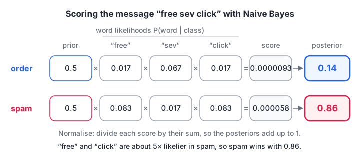
Each class gets its own chain of multiplications. Only the relative size of the final scores matters until you normalise them.
In practice the code adds logarithms instead of multiplying, because fifty probabilities like 0.01 multiplied together underflow to zero.
Naive Bayes by hand in plain Python
Here is the whole classifier, written with counts only:
from collections import Counter
import math

msgs = [("send 2 kg sev tomorrow", "order"), ("need 1 kg mixture and sev", "order"),
        ("deliver namkeen to vijay nagar", "order"), ("please send ratlami sev", "order"),
        ("3 kg bhujia for party", "order"), ("you won free recharge click link", "spam"),
        ("free gift claim now click", "spam"), ("loan approved click link now", "spam"),
        ("win free cashback today", "spam"), ("click to claim free voucher", "spam")]

words = {c: Counter() for c in ("order", "spam")}
for text, label in msgs:
    words[label].update(text.split())
vocab = set(words["order"]) | set(words["spam"])

def posterior(text, alpha=1.0):
    logs = {}
    for c in words:
        total = sum(words[c].values())
        logs[c] = math.log(0.5)                                   # prior: 5 of 10 messages
        for w in text.split():
            p = (words[c][w] + alpha) / (total + alpha * len(vocab))   # smoothed likelihood
            logs[c] += math.log(p)
    m = max(logs.values())
    expd = {c: math.exp(v - m) for c, v in logs.items()}
    return {c: round(v / sum(expd.values()), 3) for c, v in expd.items()}

print("free sev click ->", posterior("free sev click"))
print("2 kg sev       ->", posterior("2 kg sev"))
print("P(sev | order) =", round((words["order"]["sev"] + 1) / (sum(words["order"].values()) + len(vocab)), 3))
print("P(sev | spam)  =", round((words["spam"]["sev"] + 1) / (sum(words["spam"].values()) + len(vocab)), 3))
"free sev click" comes out about 0.86 spam, because two strong spam words outvote one order word. "2 kg sev" is about 0.97 order. The last two lines show why: "sev" is roughly four times as likely in an order as in spam.
What is Laplace smoothing in Naive Bayes?
"sev" never appears in the spam training messages. Without any correction, P(sev | spam) would be exactly 0, and because Naive Bayes multiplies, that single zero would wipe out the spam score however many spam words the message contained. This is the zero-frequency problem.
Laplace (additive) smoothing adds a small pseudo-count, alpha, to every word count in every class. With alpha = 1, a word seen zero times in spam is treated as if it was seen once.
That is the + alpha in the code above, and the alpha parameter of MultinomialNB, BernoulliNB, ComplementNB and CategoricalNB. Values from 0.01 to 1 are common for text; choose with cross-validation.
Quick check
In a spam filter, the word "lottery" never appeared in any non-spam training message. What does Laplace smoothing do?
Smoothing adds alpha to every count, so an unseen word can't force a class score to exactly zero.
Why is Naive Bayes called "naive"?
The independence assumption says that, within spam, seeing "click" tells you nothing about "link". In real spam the two travel together, so the assumption is false.
The damage shows up in the probabilities, not always in the predictions. When two features carry the same information, Naive Bayes counts that evidence twice and becomes more confident than it should be. The next block copies one useful feature five times:
import numpy as np
from sklearn.naive_bayes import GaussianNB
from sklearn.model_selection import train_test_split

rng = np.random.default_rng(1)
n = 600
y = rng.integers(0, 2, n)
signal = y * 1.0 + rng.normal(0, 1, n)            # one weakly useful feature
noise = rng.normal(0, 1, (n, 2))                  # two useless ones

X_once = np.column_stack([signal, noise])
X_copies = np.column_stack([np.tile(signal[:, None], 5), noise])   # same signal, 5 copies

for name, X in [("signal once", X_once), ("signal x5", X_copies)]:
    Xtr, Xte, ytr, yte = train_test_split(X, y, test_size=0.3, random_state=0)
    nb = GaussianNB().fit(Xtr, ytr)
    proba = nb.predict_proba(Xte)[:, 1]
    print(f"{name:12s} accuracy {nb.score(Xte, yte):.3f} | "
          f"mean confidence {np.maximum(proba, 1 - proba).mean():.3f}")
Accuracy barely moves, staying at about 0.71, because the ranking of the two classes hardly changes. But the average confidence jumps from about 0.67 to about 0.89. The model now claims to be sure about predictions it gets wrong almost a third of the time.
So treat predict_proba from Naive Bayes as a ranking score, not a calibrated probability. If you need trustworthy probabilities, wrap the model in CalibratedClassifierCV.
Quick check
You duplicate a feature three times. What usually happens to a Naive Bayes model?
The independence assumption makes the model count the same evidence several times, inflating its confidence.
Types of Naive Bayes classifiers
The variants differ in how they model P(feature | class), which depends on what your features look like:
| Variant | Feature type | Likelihood model | Typical use |
|---|---|---|---|
MultinomialNB |
Counts (word counts, TF-IDF) | Multinomial over the vocabulary | Spam filters, news topics, support tickets |
ComplementNB |
Counts, imbalanced classes | Learns from the other classes' counts | Text with one dominant class |
BernoulliNB |
Binary present/absent | Bernoulli per feature, absence counts too | Short texts, yes/no survey answers |
GaussianNB |
Continuous numbers | Normal curve per feature per class | Sensor readings, measurements |
CategoricalNB |
Categories encoded as integers | Frequency table per category | City, payment mode, product type |
GaussianNB is worth picturing. For each class it fits one bell curve per feature, using that class's mean and spread. A new value is scored by how tall each class's curve is at that point.
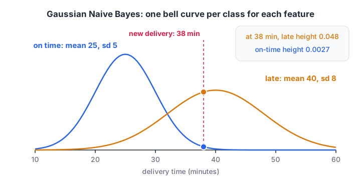
For a delivery-time feature, the late class has a wider, right-shifted curve. At 38 minutes the late curve is taller, so that feature votes late.
Quick check
Which Naive Bayes variant fits continuous features like temperature and delivery time?
GaussianNB models each feature within each class as a normal distribution with its own mean and variance.
Naive Bayes for text classification in scikit-learn
Text is where Naive Bayes shines. CountVectorizer turns each message into word counts, and MultinomialNB learns from them. Putting both in a pipeline keeps the vocabulary inside each training fold.
from sklearn.feature_extraction.text import CountVectorizer
from sklearn.naive_bayes import MultinomialNB
from sklearn.pipeline import make_pipeline
import numpy as np

texts = ["send 2 kg sev tomorrow", "need 1 kg mixture and sev", "deliver namkeen to vijay nagar",
         "please send ratlami sev", "3 kg bhujia for party", "half kg khatta meetha please",
         "is shop open sunday", "send same order as last week",
         "you won free recharge click link", "free gift claim now click", "loan approved click link now",
         "win free cashback today", "click to claim free voucher", "your kyc expired click to update",
         "congratulations you are selected claim prize", "earn money from home click"]
labels = ["order"] * 8 + ["spam"] * 8

model = make_pipeline(CountVectorizer(), MultinomialNB(alpha=0.5)).fit(texts, labels)
new = ["2 kg sev and bhujia", "claim your free sev", "click link for kyc"]
for msg, p in zip(new, model.predict_proba(new)):
    print(f"{msg:22s} P(order)={p[0]:.2f}  P(spam)={p[1]:.2f}")

vec, nb = model.named_steps["countvectorizer"], model.named_steps["multinomialnb"]
vocab = vec.get_feature_names_out()
ratio = nb.feature_log_prob_[1] - nb.feature_log_prob_[0]      # log P(w|spam) - log P(w|order)
print("most spammy words:", list(vocab[np.argsort(ratio)[-5:][::-1]]))
"claim your free sev" lands on the spam side even though it mentions sev, because "claim" and "free" carry more weight. The last line reads the learned model directly: the words with the highest spam-to-order likelihood ratio are the model's main evidence, which makes Naive Bayes easy to explain to a shop owner.
A real inbox needs thousands of messages and often TfidfVectorizer; feature engineering covers building such features.
When should you use Naive Bayes?
Naive Bayes trains by counting, in one pass with no iterations, so it handles millions of messages on a laptop. Each likelihood is estimated on its own, which also lets it reach decent accuracy from a few hundred labelled rows.
Its ceiling is lower than that of models which learn how features interact. On large tabular datasets, logistic regression or tree ensembles usually overtake it. Use Naive Bayes as the first baseline for any text problem and keep it in production when it is close enough.
| Strengths | Weaknesses |
|---|---|
| Trains in one pass, predicts instantly | Probabilities are overconfident |
| Works with small training sets | Plateaus early on large tabular data |
| Handles thousands of word features well | Correlated features are double-counted |
| Easy to explain with word likelihoods | Unseen categories need smoothing |
| No feature scaling needed | GaussianNB assumes bell-shaped features |
Common Naive Bayes mistakes
- Using GaussianNB on word counts. Counts are not bell-shaped. Use MultinomialNB or ComplementNB for text.
- Setting alpha to 0. One unseen word zeroes a whole class. Keep alpha above zero and tune it.
- Trusting predict_proba as a real probability. It ranks well but is badly calibrated, especially with correlated features.
- Feeding negative values to MultinomialNB. It expects counts or TF-IDF, so standardised features with negative numbers raise an error.
- Fitting the vectorizer on all data before splitting. Put it inside a pipeline so test words don't leak into the vocabulary.
To build a full text classifier with a mentor checking each step, look at the machine learning programme at Debugshala in Indore. Next in this series is support vector machines, a model that draws the widest possible boundary between classes. To revise first, solve Naive Bayes practice MCQs on Debugshala Test.
Key takeaways
- Naive Bayes multiplies a class prior by one likelihood per feature and picks the class with the largest result.
- The "naive" part is assuming features are independent within each class; rankings survive this better than probabilities do.
- Pick the variant by feature type: Multinomial or Complement for counts, Bernoulli for binary, Gaussian for continuous, Categorical for categories.
- Laplace smoothing (alpha) prevents zero probabilities; tune it with cross-validation.
- It is fast and explainable: the go-to first baseline for text.
FAQ
What is Naive Bayes used for in real life?
Naive Bayes is used mostly for text: spam filtering, sorting support tickets, tagging news articles by topic and quick sentiment checks. It suits these jobs because text has thousands of word features, and Naive Bayes handles them with simple counts, trains in seconds and stays reasonably accurate even with a few hundred labelled examples.
Is Naive Bayes better than logistic regression?
Neither is better everywhere. Naive Bayes often wins with very small training sets and high-dimensional text, because it needs fewer rows to estimate its counts. Logistic regression usually wins once you have more data, since it can account for correlated features. A sensible habit is to try both with cross-validation.
Does Naive Bayes need feature scaling?
No. Naive Bayes estimates probabilities for each feature separately within each class, so changing a feature's units does not change which class wins. GaussianNB learns each feature's own mean and variance, and MultinomialNB works on raw counts. Scaling is harmless for GaussianNB but can break MultinomialNB if it creates negative values.
Can I learn Naive Bayes and text classification at Debugshala in Indore?
Yes. Naive Bayes and the other core classifiers are part of Debugshala's Machine Learning course, taught offline at the Old Palasia campus in Indore in English and Hindi. Fresh graduates and learners from non-IT backgrounds are welcome, and you can attend a free demo class before paying anything.
From the team behind this site
Go further with the Data Science & AI Course at Debugshala
These tutorials are written by Debugshala, a training and placement institute at Old Palasia, Indore. The classroom course adds live mentoring, real projects and interview preparation.
- Offline classes at Old Palasia, Indore
- Free demo class before you pay
- Non-IT, fresher and year-gap friendly
- Placement assistance
700+ students placed · 200+ hiring partners · 4.9★ Google rating
