

Linear Regression Explained: Least Squares to scikit-learn
Linear regression explained with rickshaw fares and rent data: least squares, coefficients, gradient descent, residual checks and assumptions, in Python.
Suppose you take auto-rickshaws around Indore all month and note every ride: 1.5 km from Palasia to the station cost ₹48, the 9 km run to the airport cost ₹150. Plot distance against fare and the dots fall almost on a straight line.
From that line you can read two numbers. Where it starts, at zero kilometres, is roughly the minimum charge. How steeply it climbs is the price per kilometre. With those two numbers you can predict the fare for a ride you haven't taken yet.
You have just done linear regression in your head.
What is linear regression?
Map the rides to the terms:
- Distance is the feature (input, also called the independent variable or x).
- Fare is the target (output, dependent variable or y).
- The starting value is the intercept b.
- The price per kilometre is the slope or coefficient w.
- The gap between a real fare and the line's fare is a residual.
Linear regression is a supervised learning algorithm that models a numeric target as a straight-line (linear) combination of input features, choosing the coefficients that minimise the sum of squared differences between predicted and actual values.
With one feature it is simple linear regression: y = b + w·x. With several it is multiple linear regression: y = b + w1·x1 + w2·x2 + … + wp·xp.
It is the first model in the supervised learning part of this series and the base for logistic regression, which comes next. Code here targets scikit-learn 1.7 and NumPy 2.x.
How does linear regression find the best line?
Infinitely many lines pass near the dots. Linear regression picks the one with the smallest sum of squared residuals, a method called ordinary least squares (OLS).
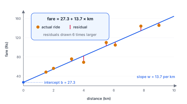
Each vertical segment is a residual. Least squares chooses the intercept and slope that make the sum of their squares as small as possible.
Why squared? Squaring makes every error positive, so misses above and below the line don't cancel. It also punishes one large miss more than several small ones. And it gives a neat formula for simple regression: slope = covariance(x, y) / variance(x).
import numpy as np

# 8 auto-rickshaw rides in Indore: distance (km) and fare paid (rupees)
km   = np.array([1.5, 2.0, 3.2, 4.0, 5.5, 6.1, 7.8, 9.0])
fare = np.array([ 48,  55,  72,  80, 104, 110, 136, 150])

# least squares by hand: slope = cov(x, y) / var(x)
slope = np.sum((km - km.mean()) * (fare - fare.mean())) / np.sum((km - km.mean()) ** 2)
intercept = fare.mean() - slope * km.mean()
print(f"fare = {intercept:.1f} + {slope:.1f} x km")

pred = intercept + slope * km
print("residuals:", np.round(fare - pred, 1))
print("sum of squared residuals:", round(float(np.sum((fare - pred) ** 2)), 1))
print("np.polyfit agrees:", np.round(np.polyfit(km, fare, 1), 1))
print("predicted fare for 5 km:", round(intercept + slope * 5))
The fitted rule is fare ≈ ₹27.3 + ₹13.7 per km, and a 5 km ride should cost about ₹96. Every residual is within ₹2.2, which tells you the straight line suits this data.
For several features, the same idea is solved with matrices, the normal equation (XᵀX)⁻¹Xᵀy, which linear algebra for data science walks through. You rarely compute it yourself, because scikit-learn does.
Quick check
What does ordinary least squares minimise?
Plain residuals above and below the line would cancel out, so OLS minimises their squares.
Multiple linear regression with scikit-learn
Real targets depend on several things. Here is a rent model for 300 synthetic flats, with area, distance from the city centre and floor number. Follow the standard steps:
- Build a table of features and a target column.
- Split into training and test sets.
- Fit
LinearRegressionon the training set. - Read
intercept_andcoef_. - Score on the test set and predict for new rows.
import numpy as np
import pandas as pd
from sklearn.linear_model import LinearRegression
from sklearn.model_selection import train_test_split
from sklearn.metrics import r2_score, mean_absolute_error

rng = np.random.default_rng(8)
n = 300
flats = pd.DataFrame({
    "area_sqft": rng.integers(450, 1800, n),
    "km_to_centre": rng.uniform(1, 15, n).round(1),
    "floor": rng.integers(0, 12, n),
})
# monthly rent in rupees: the "true" rule plus noise
rent = (2000 + 11 * flats.area_sqft - 350 * flats.km_to_centre
        + 150 * flats.floor + rng.normal(0, 1500, n))

X_tr, X_te, y_tr, y_te = train_test_split(flats, rent, test_size=0.25, random_state=0)
model = LinearRegression().fit(X_tr, y_tr)
print("intercept:", round(model.intercept_))
for name, c in zip(flats.columns, model.coef_):
    print(f"  {name:>13}: {c:8.1f} rupees per unit")
pred = model.predict(X_te)
print(f"test R2 = {r2_score(y_te, pred):.3f}, MAE = Rs {mean_absolute_error(y_te, pred):,.0f}")
new = pd.DataFrame({"area_sqft": [1000], "km_to_centre": [4.0], "floor": [3]})
print(f"rent for a 1,000 sq ft flat, 4 km out, 3rd floor: Rs {model.predict(new)[0]:,.0f}")
The model recovers the hidden rule closely: about ₹10.7 per extra square foot, −₹358 for each kilometre farther out, and +₹111 per floor. Test R² of 0.855 means it explains about 86% of the variation in rent; MAE says a typical miss is ₹1,344. The metrics are explained in model evaluation metrics.
How to interpret linear regression coefficients
A coefficient is the expected change in the target for a one-unit rise in that feature, holding the other features constant. Three cautions:
- Units matter. ₹10.7 per square foot and ₹358 per kilometre can't be compared directly. Standardise features first if you want to rank their importance.
- Correlated features blur meaning. If area and number of rooms move together, their coefficients share credit unpredictably, the problem that ridge and lasso regularization solves.
- Coefficients show association, not cause. Floor number may stand in for a lift or a better view.
Quick check
A model predicts rent = 2000 + 11 × area_sqft. What is the predicted rent for an 800 sq ft flat?
2000 + 11 × 800 = 2000 + 8800 = 10,800.
Training linear regression with gradient descent
The formula works well for small and medium data. For very large data, and for neural networks, models are trained by gradient descent instead: start with any line, measure the error, nudge the slope and intercept in the direction that reduces the error, repeat.
import numpy as np

km   = np.array([1.5, 2.0, 3.2, 4.0, 5.5, 6.1, 7.8, 9.0])
fare = np.array([ 48,  55,  72,  80, 104, 110, 136, 150])

w, b = 0.0, 0.0                 # start with a flat line at zero
lr = 0.02                       # learning rate: size of each step
for step in range(1, 3001):
    pred = w * km + b
    error = pred - fare
    grad_w = 2 * np.mean(error * km)        # slope of the MSE with respect to w
    grad_b = 2 * np.mean(error)             # ... and with respect to b
    w -= lr * grad_w
    b -= lr * grad_b
    if step in (1, 10, 100, 1000, 3000):
        print(f"step {step:4d}: fare = {b:5.1f} + {w:5.2f} x km | MSE {np.mean(error ** 2):8.1f}")
After about 1,000 steps the line settles at the same ₹27.3 + ₹13.7 per km that least squares gave directly. Set the learning rate too high (try 0.05) and the numbers blow up instead. Optimisers that tune this step size are covered in gradient descent optimizers.
What are the assumptions of linear regression?
Linear regression gives trustworthy predictions and coefficients when these hold reasonably well:
| Assumption | Meaning | How to check | Fix if broken |
|---|---|---|---|
| Linearity | The target changes in a straight line with each feature | Residuals show no curve | Add squared or log features |
| Independence | Errors of different rows are unrelated | Think about the data source; time order | Time series models, grouped data methods |
| Constant variance | Residual spread is similar across predictions | No funnel shape in residuals | Log-transform the target |
| No strong multicollinearity | Features aren't near copies | Correlation matrix, VIF | Drop one, or use ridge |
| Roughly normal residuals | Mainly for confidence intervals and p-values | Histogram of residuals | Usually fine with enough data |
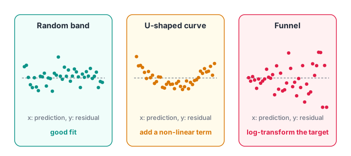
Plot residuals against predictions. A shapeless band is what you want; a curve or a funnel tells you which assumption is broken.
Checking residuals for a curve
AC sales climb slowly on warm days and shoot up on very hot ones. A straight line misses that bend, and the residuals reveal it:
import numpy as np
from sklearn.linear_model import LinearRegression

rng = np.random.default_rng(2)
# AC sales vs temperature: sales take off sharply on very hot days
temp = rng.uniform(24, 46, 200)
sales = 5 + 0.04 * (temp - 24) ** 2.2 + rng.normal(0, 4, 200)

X_line = temp.reshape(-1, 1)
X_curve = np.column_stack([temp, temp ** 2])        # add a squared feature
bands = [(24, 30), (30, 36), (36, 42), (42, 46)]
for name, X in [("straight line", X_line), ("with temp^2", X_curve)]:
    model = LinearRegression().fit(X, sales)
    resid = sales - model.predict(X)
    means = [resid[(temp >= lo) & (temp < hi)].mean() for lo, hi in bands]
    print(f"{name:>13}: R2 {model.score(X, sales):.3f} | mean residual per band:",
          np.round(means, 1))
The straight line's average residual goes positive, negative, negative, positive across the temperature bands: the U shape of a missed curve. Adding temp² brings every band close to zero and lifts R² from 0.78 to 0.87.
The model is still "linear" because it is linear in its coefficients, even though the fitted line now bends. More ideas for such features are in feature engineering.
On your own machine, a residual plot takes three lines:
import matplotlib.pyplot as plt
plt.scatter(model.predict(X), resid, s=12)
plt.axhline(0, color="grey"); plt.xlabel("predicted"); plt.ylabel("residual"); plt.show()
Quick check
Residuals form a clear U shape when plotted against temperature. What should you try?
A U-shaped residual pattern means the relationship is curved, which a squared term can capture.
Common linear regression mistakes
- Extrapolating far outside the data. A fare line fitted on 1 to 9 km may be wrong for a 40 km trip.
- Reading coefficients as importance without scaling. Compare standardised coefficients or use permutation importance.
- Ignoring outliers. Squared error lets one extreme flat pull the whole line; check outliers first.
- Feeding raw categories as numbers. Encode city or flat type with one-hot encoding, not 1, 2, 3.
- Judging by training R² only. Always report test R², MAE or RMSE.
Linear regression is where most learners first connect statistics to prediction, and Debugshala's beginner-friendly machine learning course starts its supervised learning work here. If you want the wider path through Python, statistics and ML, see Debugshala's wider data science & AI course. To check yourself, solve regression MCQs on Debugshala Test.
Key takeaways
- Linear regression predicts a number as an intercept plus a weighted sum of features.
- Least squares picks the coefficients that minimise the sum of squared residuals; gradient descent reaches the same answer step by step.
- A coefficient is the change in the target per one-unit rise in a feature, with the others held fixed.
- Check residuals: curves mean missing non-linear terms, funnels mean changing variance.
- Evaluate on test data with R², MAE and RMSE, and regularize when features are many or correlated.
FAQ
What is linear regression in simple words?
Linear regression draws the straight line (or flat surface, with several inputs) that best fits your data points, then uses it to predict a number. For example, it can learn that a rickshaw fare is about ₹27 plus ₹13.7 per kilometre, and predict the fare of any new ride from its distance.
What is the difference between simple and multiple linear regression?
Simple linear regression uses one input feature, such as distance, to predict the target. Multiple linear regression uses two or more features, such as area, distance and floor, each with its own coefficient. The fitting method, least squares, is the same for both.
What is a good R² value for linear regression?
It depends on the field. In controlled physical measurements R² above 0.9 is common, while for people's behaviour, such as spending or churn, 0.3 to 0.6 can still be useful. Compare R² with a simple baseline and always measure it on test data, not training data.
Is linear regression machine learning or statistics?
Both. Statistics uses linear regression mainly to explain relationships, with confidence intervals and p-values. Machine learning uses the same model mainly to predict new values, judged on held-out data. scikit-learn focuses on prediction; the statsmodels library gives the classical statistical summary.
Can I learn linear regression at Debugshala in Indore?
Yes. Linear regression is taught in Debugshala's Machine Learning course at the Old Palasia campus in Indore, with offline classes in English and Hindi. Fresh graduates, non-IT learners and people with a year gap can join, and a free demo class is available before you pay anything.
From the team behind this site
Go further with the Data Science & AI Course at Debugshala
These tutorials are written by Debugshala, a training and placement institute at Old Palasia, Indore. The classroom course adds live mentoring, real projects and interview preparation.
- Offline classes at Old Palasia, Indore
- Free demo class before you pay
- Non-IT, fresher and year-gap friendly
- Placement assistance
700+ students placed · 200+ hiring partners · 4.9★ Google rating
