

Handling Imbalanced Data: Class Weights, SMOTE and Thresholds
Handle imbalanced data in machine learning: why accuracy fails, class weights, oversampling, undersampling, SMOTE, threshold tuning and PR-AUC, with code.
Picture a cooperative bank in Indore that approves 4,000 small business loans a year. About 120 of those borrowers will default. The credit officer builds a model, and it reports 97% accuracy on day one.
Then someone asks how many of the 120 defaulters it would have flagged. The honest answer is very few. A model that approves everyone is already right 97% of the time, so the training process found little reason to learn what a defaulter looks like.
That is the imbalanced data problem. The rare class is usually the one you care about most.
What is imbalanced data in machine learning?
Map the bank to the terms:
- Defaulters are the minority class (also called the positive class), here about 3% of rows.
- Repaying borrowers are the majority class.
- The ratio, about 1:32 here, is the imbalance ratio.
- Approving everyone is the majority-class baseline, and its accuracy is the bar any model must beat on other metrics.
Imbalanced data is a classification dataset in which one class has far fewer examples than the others, which biases models towards predicting the majority class and makes accuracy a misleading measure of performance.
You meet it everywhere: card fraud, machine failures, rare diseases, customer churn, spam in a work inbox, defects on a factory line. This lesson closes the foundations part of the series, after feature selection. The code here uses scikit-learn 1.7, and the metrics come from model evaluation metrics.
Why does accuracy fail on imbalanced data?
Build a synthetic version of the bank's data with about 3% defaults and compare a do-nothing baseline with a real model:
import numpy as np
from sklearn.datasets import make_classification
from sklearn.model_selection import train_test_split
from sklearn.linear_model import LogisticRegression
from sklearn.metrics import accuracy_score, recall_score, precision_score

# 4,000 loan applications, about 3% default (label 1)
X, y = make_classification(n_samples=4000, n_features=8, n_informative=4,
                           weights=[0.97], flip_y=0.005, class_sep=1.0, random_state=7)
X_tr, X_te, y_tr, y_te = train_test_split(X, y, test_size=0.25, stratify=y, random_state=0)
print("defaults in test set:", int(y_te.sum()), "of", len(y_te))

never = np.zeros_like(y_te)                       # "nobody defaults"
model = LogisticRegression().fit(X_tr, y_tr)
pred = model.predict(X_te)
for name, p in [("always 'no default'", never), ("logistic regression", pred)]:
    print(f"{name:>20}: accuracy {accuracy_score(y_te, p):.3f} | "
          f"recall {recall_score(y_te, p):.2f} | "
          f"precision {precision_score(y_te, p, zero_division=0):.2f}")
The baseline scores 96.9% accuracy and catches nothing. The logistic regression scores 97.8% and catches only 39% of defaulters (recall 0.39). Its flags are usually right (precision 0.80), but it lets 19 of 31 defaulters through.
Two habits fix the measurement before you fix the model:
- Stratify every split with
stratify=yand useStratifiedKFold, so each part has the same 3%. Cross-validation explains why. - Report minority-class metrics: recall, precision, F1 and PR-AUC (average precision). PR-AUC summarises precision and recall across all thresholds and, unlike ROC-AUC, is not flattered by a huge pile of easy negatives.
Quick check
A dataset has 990 genuine and 10 fraud transactions. A model predicts "genuine" for all of them. What is its accuracy and fraud recall?
It is right on all 990 genuine rows (99% accuracy) but catches none of the 10 frauds, so recall is 0.
What are the techniques for handling imbalanced data?
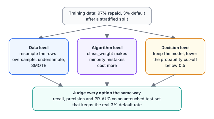
You can rebalance the data, tell the algorithm that minority mistakes cost more, or change where you cut the predicted probability. All three are judged with recall, precision and PR-AUC.
| Technique | Level | What it does | Watch out for |
|---|---|---|---|
| Class weights | Algorithm | Makes minority errors cost more in the loss | Not every model supports it |
| Random oversampling | Data | Repeats minority rows | Overfitting to repeated rows |
| Random undersampling | Data | Drops majority rows | Throws away information |
| SMOTE | Data | Creates synthetic minority rows between neighbours | Noise and overlap get amplified |
| Threshold moving | Decision | Lowers the probability cut-off for "yes" | Needs a validation set to choose it |
| More minority data | Data | Collect or label more rare cases | Slow, but often the best fix |
Class weights: the simplest fix
Most scikit-learn classifiers accept class_weight. Setting it to "balanced" weights each class by n_samples / (n_classes × class_count), so every defaulter counts about 16 times as much as a repaying borrower.
import numpy as np
from sklearn.datasets import make_classification
from sklearn.model_selection import train_test_split
from sklearn.linear_model import LogisticRegression
from sklearn.metrics import recall_score, precision_score, f1_score, average_precision_score

X, y = make_classification(n_samples=4000, n_features=8, n_informative=4,
                           weights=[0.97], flip_y=0.005, class_sep=1.0, random_state=7)
X_tr, X_te, y_tr, y_te = train_test_split(X, y, test_size=0.25, stratify=y, random_state=0)

for cw in [None, "balanced", {0: 1, 1: 10}]:
    m = LogisticRegression(class_weight=cw).fit(X_tr, y_tr)
    p = m.predict(X_te)
    ap = average_precision_score(y_te, m.predict_proba(X_te)[:, 1])
    print(f"class_weight={str(cw):>16}: recall {recall_score(y_te, p):.2f} | "
          f"precision {precision_score(y_te, p):.2f} | F1 {f1_score(y_te, p):.2f} | PR-AUC {ap:.2f}")
print("balanced weight for class 1:", round(len(y_tr) / (2 * y_tr.sum()), 1))
Balanced weights lift recall from 0.39 to 0.90, but precision falls to 0.14: the model now flags about six good borrowers for every real defaulter. A milder weight of 10 lands in between.
Notice PR-AUC does not go up. Weighting did not make the model better at ranking risky borrowers; it moved the cut-off. That is the key insight of this topic.
Oversampling, undersampling and SMOTE
Resampling changes the training data instead of the loss. The one rule you must never break: resample only the training data, after the split. The test set must keep the real-world 3%.
import numpy as np
from sklearn.datasets import make_classification
from sklearn.model_selection import train_test_split
from sklearn.linear_model import LogisticRegression
from sklearn.metrics import recall_score, precision_score
from sklearn.utils import resample

X, y = make_classification(n_samples=4000, n_features=8, n_informative=4,
                           weights=[0.97], flip_y=0.005, class_sep=1.0, random_state=7)
X_tr, X_te, y_tr, y_te = train_test_split(X, y, test_size=0.25, stratify=y, random_state=0)
maj, mino = X_tr[y_tr == 0], X_tr[y_tr == 1]

# oversample: copy minority rows (with replacement) until classes match
mino_up = resample(mino, n_samples=len(maj), replace=True, random_state=0)
X_over, y_over = np.vstack([maj, mino_up]), np.r_[np.zeros(len(maj)), np.ones(len(maj))]
# undersample: keep only as many majority rows as there are minority rows
maj_down = resample(maj, n_samples=len(mino), replace=False, random_state=0)
X_under, y_under = np.vstack([maj_down, mino]), np.r_[np.zeros(len(mino)), np.ones(len(mino))]

for name, (Xs, ys) in {"original": (X_tr, y_tr), "oversampled": (X_over, y_over),
                       "undersampled": (X_under, y_under)}.items():
    p = LogisticRegression().fit(Xs, ys).predict(X_te)       # test set untouched
    print(f"{name:>12}: {len(ys):5d} training rows | recall {recall_score(y_te, p):.2f} "
          f"| precision {precision_score(y_te, p):.2f}")
Both resampled versions behave almost exactly like balanced class weights: recall around 0.9, precision around 0.14. Undersampling got there with only 186 training rows, which is fast but wastes 2,800 real examples. With flexible models such as deep trees, plain oversampling also invites overfitting, because the model sees the same defaulter many times.
How does SMOTE work?
SMOTE (Synthetic Minority Over-sampling Technique) creates new minority rows instead of copying old ones. For each new row it picks a minority point, picks one of its k nearest minority neighbours, and places a synthetic point at a random spot on the line between them.
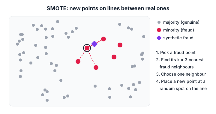
SMOTE fills the space between real fraud cases. New points never leave the region the minority class already occupies.
Here is the core idea in about ten lines of numpy:
import numpy as np
from sklearn.neighbors import NearestNeighbors

def smote(X_min, n_new, k=5, seed=0):
    """Create n_new synthetic minority rows by interpolating between neighbours."""
    rng = np.random.default_rng(seed)
    nn = NearestNeighbors(n_neighbors=k + 1).fit(X_min)
    _, idx = nn.kneighbors(X_min)                 # idx[:, 0] is the point itself
    base = rng.integers(0, len(X_min), n_new)     # random minority rows
    mate = idx[base, rng.integers(1, k + 1, n_new)]  # one of their k neighbours
    gap = rng.random((n_new, 1))                  # how far along the line to go
    return X_min[base] + gap * (X_min[mate] - X_min[base])

# 6 fraud transactions: [amount in thousand rupees, transactions in last hour]
fraud = np.array([[48, 5], [52, 6], [45, 7], [60, 6], [55, 8], [50, 4]], dtype=float)
synthetic = smote(fraud, n_new=4, k=3)
print("synthetic fraud rows:")
print(synthetic.round(1))
print("all inside the original range?",
      bool(((synthetic >= fraud.min(0)) & (synthetic <= fraud.max(0))).all()))
Notice the synthetic rows have fractional transaction counts such as 4.8. That is fine for a model but shows SMOTE assumes features are continuous. For categorical columns, the library version has SMOTENC.
In practice you use the open-source imbalanced-learn package, whose pipeline applies SMOTE only while fitting, never to validation folds:
# pip install imbalanced-learn
from imblearn.over_sampling import SMOTE
from imblearn.pipeline import Pipeline
from sklearn.linear_model import LogisticRegression
from sklearn.model_selection import StratifiedKFold, cross_val_score
from sklearn.preprocessing import StandardScaler

pipe = Pipeline([
    ("scale", StandardScaler()),
    ("smote", SMOTE(k_neighbors=5, random_state=0)),
    ("model", LogisticRegression()),
])
cv = StratifiedKFold(n_splits=5, shuffle=True, random_state=0)
print(cross_val_score(pipe, X, y, cv=cv, scoring="average_precision").mean())
Use imblearn.pipeline.Pipeline here, not scikit-learn's, because only the imbalanced-learn version knows how to skip resampling at prediction time. The imbalanced-learn documentation lists the other samplers.
Quick check
When should SMOTE be applied?
Synthetic rows must never reach validation or test data, or they leak information and inflate scores.
Threshold moving: change the decision, not the data
A classifier's predict cuts the probability at 0.5. With 3% defaults, few borrowers ever reach 0.5. Instead of rebalancing anything, you can keep the model and choose a lower cut-off on a validation set, using a business rule such as "catch at least 70% of defaulters".
import numpy as np
from sklearn.datasets import make_classification
from sklearn.model_selection import train_test_split
from sklearn.linear_model import LogisticRegression
from sklearn.metrics import precision_recall_curve

X, y = make_classification(n_samples=4000, n_features=8, n_informative=4,
                           weights=[0.97], flip_y=0.005, class_sep=1.0, random_state=7)
X_tr, X_te, y_tr, y_te = train_test_split(X, y, test_size=0.25, stratify=y, random_state=0)
X_fit, X_val, y_fit, y_val = train_test_split(X_tr, y_tr, test_size=0.3, stratify=y_tr, random_state=0)

model = LogisticRegression().fit(X_fit, y_fit)
prec, rec, thr = precision_recall_curve(y_val, model.predict_proba(X_val)[:, 1])
# business rule: catch at least 70% of defaults
ok = np.flatnonzero(rec[:-1] >= 0.70)
best_t = thr[ok[-1]]                              # highest threshold that still meets it
print(f"chosen threshold: {best_t:.3f} (default is 0.5)")

proba_te = model.predict_proba(X_te)[:, 1]
for t in [0.5, best_t]:
    p = proba_te >= t
    tp = int((p & (y_te == 1)).sum())
    print(f"threshold {t:.3f}: flagged {int(p.sum()):3d}, caught {tp} of {int(y_te.sum())} defaults")
A threshold near 0.07 makes the model flag about 100 applications and catch 24 of the 31 defaulters on the untouched test set.
If the bank's credit team can review 100 files, that is a workable plan, built without changing the training data at all. scikit-learn 1.5 and later also offer TunedThresholdClassifierCV, which searches the threshold with cross-validation, much like the searches in hyperparameter tuning. The same probability-then-threshold idea is at the heart of logistic regression, the next topic.
Which technique should you choose?
- Fix the metrics and stratify the splits.
- Try class weights or threshold moving first: they are simple and leak-proof.
- Try SMOTE or undersampling when a model has no
class_weightoption, or when training time matters. - Compare everything on PR-AUC plus precision and recall at your chosen operating point.
- If the minority class is tiny (say under 50 rows), spend effort on collecting more examples.
Quick check
After setting class_weight="balanced", recall rises from 0.4 to 0.9 but PR-AUC stays the same. What happened?
Class weights mainly shift where the model says "yes". PR-AUC, which summarises ranking across all thresholds, barely moves.
Common mistakes with imbalanced datasets
- Resampling before the split. Synthetic or copied rows leak into the test set and inflate every score.
- Reporting accuracy or ROC-AUC alone. Both can look strong while the minority class is mostly missed.
- Testing on balanced data. The test set must reflect the real class ratio, or precision will look far better than it will be in production.
- Assuming SMOTE always helps. With strong models, class weights or threshold tuning often match it with less complexity.
- Ignoring calibration. Resampling and weights distort predicted probabilities, so don't read them as real default rates without recalibrating.
Working through a fraud or churn project from metrics to threshold choice, with a mentor reviewing it, is part of a mentor-led machine learning course in Indore. To test yourself on these trade-offs, check your imbalanced-data instincts on Debugshala Test.
Key takeaways
- On imbalanced data, accuracy rewards predicting the majority class; use recall, precision, F1 and PR-AUC.
- Stratify every split and cross-validation fold.
- Class weights, resampling and threshold moving all trade precision for recall; pick the point that fits the business cost.
- Resample only the training data, and use imbalanced-learn's pipeline for SMOTE inside cross-validation.
- Keep the test set at the real-world class ratio.
FAQ
What is considered imbalanced data?
Data is usually called imbalanced when the minority class makes up less than about 20% of rows, and severely imbalanced below 1 to 5%. The exact cut-off matters less than the symptom: if a majority-class baseline already scores high accuracy, you need minority-class metrics and probably one of the fixes above.
Is SMOTE better than class weights?
Not necessarily. SMOTE and class weights often give similar results for linear models and tree ensembles, and class weights are simpler and cannot leak synthetic rows. SMOTE is useful when a model has no weighting option or when the minority region is sparse. Compare both with cross-validated PR-AUC.
Should I balance the test set?
No. The test set should keep the real class ratio that the model will face in production. Balancing it makes precision look much better than it will really be. Only the training data, inside each fold, should be resampled or reweighted.
Which metric is best for imbalanced classification?
PR-AUC (average precision) is a good single summary because it focuses on the minority class. For decisions, report precision and recall at the threshold you will actually use. F1 is useful when false positives and false negatives cost roughly the same.
Where can I learn to handle imbalanced data in Indore?
Debugshala teaches imbalanced classification as part of its Machine Learning course at the Old Palasia campus in Indore. Classes run offline in English and Hindi and accept fresh graduates, non-IT learners and people with a year gap. You can book a free demo class before paying.
From the team behind this site
Go further with the Data Science & AI Course at Debugshala
These tutorials are written by Debugshala, a training and placement institute at Old Palasia, Indore. The classroom course adds live mentoring, real projects and interview preparation.
- Offline classes at Old Palasia, Indore
- Free demo class before you pay
- Non-IT, fresher and year-gap friendly
- Placement assistance
700+ students placed · 200+ hiring partners · 4.9★ Google rating
