

Hyperparameter Tuning: Grid, Random and Bayesian Search
Hyperparameter tuning in scikit-learn: GridSearchCV vs RandomizedSearchCV, a hands-on Bayesian optimisation loop, Optuna, and a practical tuning workflow.
Imagine you run a chai stall near Sarafa Bazaar and want the perfect cup. You can change three things: how many spoons of tea leaves, how much sugar, and how long it boils. The milk and leaves do their own chemistry once they are in the pan. Your job is to pick the dials before you start.
You could brew every combination of 3 leaf amounts, 4 sugar levels and 5 boiling times. That is 60 cups. Or you could brew 15 random combinations and see which region tastes best. Or you could taste each cup and let it guide the next one: "too bitter, so less boiling next time."
Those three habits are grid search, random search and Bayesian search.
What is hyperparameter tuning?
Map the chai stall to machine learning:
- The chemistry in the pan is training. The model learns its own parameters, such as regression coefficients or tree split points, from the data.
- The dials you set before brewing are hyperparameters: tree depth, number of neighbours, penalty strength, learning rate.
- Tasting a cup is scoring one setting with cross-validation.
- Choosing which cups to brew is the search strategy.
Hyperparameter tuning is the process of searching for the hyperparameter values, the settings fixed before training, that give a model the best performance on validation data, usually measured with cross-validation.
| Parameters | Hyperparameters | |
|---|---|---|
| Who sets them | The training algorithm | You, before training |
| Examples | Coefficients, tree split thresholds, neural network weights | max_depth, C, alpha, n_neighbors, learning rate |
| Found by | Fitting on training data | Search with cross-validation |
| Stored in scikit-learn as | Attributes ending in _, such as coef_ |
Constructor arguments, such as SVC(C=10) |
Code in this article uses scikit-learn 1.7.
Quick check
Which of these is a hyperparameter, not a learned parameter?
k is chosen before training. Coefficients and split thresholds are learned from the data during fitting.
Why do hyperparameters matter so much?
The same algorithm can underfit or overfit depending only on its settings. A decision tree's max_depth is a good example, building on the decision trees tutorial:
from sklearn.datasets import make_classification
from sklearn.model_selection import cross_val_score
from sklearn.tree import DecisionTreeClassifier

X, y = make_classification(n_samples=400, n_features=10, n_informative=4,
                           flip_y=0.08, random_state=7)

for depth in [1, 2, 3, 5, 8, 12, None]:
    tree = DecisionTreeClassifier(max_depth=depth, random_state=0)
    score = cross_val_score(tree, X, y, cv=5).mean()
    print(f"max_depth={str(depth):>4}: CV accuracy {score:.3f}")

tree = DecisionTreeClassifier(max_depth=5, random_state=0).fit(X, y)
print("learned parameters (split rules):", tree.tree_.node_count, "nodes")
Shallow trees around depth 3 score best, near 0.81. Unlimited depth drops to about 0.79 because the tree starts memorising noise. You chose max_depth; the tree then learned its own 43 nodes. That split is exactly the parameter versus hyperparameter difference.
How does grid search work?
Grid search tries every combination from lists of values you provide, scores each with cross-validation, and keeps the best. Follow these steps:
- Put preprocessing and the model in a pipeline so scaling happens inside each fold.
- Write a dictionary of hyperparameter names and the values to try.
- Pass both to
GridSearchCVwith acvand ascoringmetric. - Call
fiton the training set only. - Read
best_params_andbest_score_, then score once on the test set.
from sklearn.datasets import make_classification
from sklearn.model_selection import GridSearchCV, train_test_split
from sklearn.pipeline import make_pipeline
from sklearn.preprocessing import StandardScaler
from sklearn.svm import SVC

X, y = make_classification(n_samples=400, n_features=10, n_informative=4,
                           flip_y=0.08, random_state=7)
X_tr, X_te, y_tr, y_te = train_test_split(X, y, test_size=0.25, stratify=y, random_state=0)

pipe = make_pipeline(StandardScaler(), SVC())
grid = {"svc__C": [0.1, 1, 10, 100],
        "svc__gamma": [0.001, 0.01, 0.1, 1]}
search = GridSearchCV(pipe, grid, cv=5, scoring="accuracy")
search.fit(X_tr, y_tr)

n = len(search.cv_results_["params"])
print("combinations tried:", n, "| model fits:", n * 5 + 1)
print("best settings:", search.best_params_)
print(f"best CV accuracy: {search.best_score_:.3f}")
print(f"test accuracy of the refitted best model: {search.score(X_te, y_te):.3f}")
Sixteen combinations times five folds is 80 fits, plus one final refit of the winner on all training rows. The names use the pipeline step, two underscores, then the argument: svc__C. Notice the test score (0.87) is a little below the best CV score (0.90). That is normal, because picking the best of 16 slightly flatters the winner.
The weakness is cost. Grid size multiplies: five hyperparameters with five values each is 3,125 combinations, or 15,625 fits with 5-fold CV.
Quick check
A grid has 4 values of C, 5 values of gamma and 3 kernels, with 5-fold CV. How many fits does the search run, ignoring the final refit?
4 × 5 × 3 = 60 combinations, each fitted 5 times, gives 300 fits.
Grid search vs random search: which is better?
Random search draws a fixed number of combinations from ranges or distributions. It sounds careless, but it usually finds good settings faster.
The reason is that most models have only one or two hyperparameters that really matter. A 3 × 3 grid tests just three distinct values of the important one. Nine random points test nine distinct values of it.
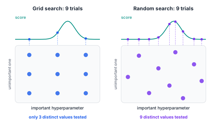
Same budget of nine trials. When only the horizontal hyperparameter matters, random search explores it three times more thoroughly than the grid does.
from scipy.stats import loguniform
from sklearn.datasets import make_classification
from sklearn.model_selection import RandomizedSearchCV, train_test_split
from sklearn.pipeline import make_pipeline
from sklearn.preprocessing import StandardScaler
from sklearn.svm import SVC

X, y = make_classification(n_samples=400, n_features=10, n_informative=4,
                           flip_y=0.08, random_state=7)
X_tr, X_te, y_tr, y_te = train_test_split(X, y, test_size=0.25, stratify=y, random_state=0)

pipe = make_pipeline(StandardScaler(), SVC())
space = {"svc__C": loguniform(0.01, 1000),        # any value, spread on a log scale
         "svc__gamma": loguniform(0.0001, 10)}
search = RandomizedSearchCV(pipe, space, n_iter=16, cv=5, random_state=0)
search.fit(X_tr, y_tr)

best = search.best_params_
print(f"best C = {best['svc__C']:.3g}, best gamma = {best['svc__gamma']:.3g}")
print(f"best CV accuracy: {search.best_score_:.3f}")
print(f"test accuracy:    {search.score(X_te, y_te):.3f}")
With the same budget of 16 combinations, random search lands on C ≈ 1.3 and gamma ≈ 0.17. It matches the grid's CV score and does slightly better on test, without anyone choosing the candidate values. loguniform spreads samples evenly across orders of magnitude, which suits hyperparameters like C, alpha and learning rate.
| Method | How it picks trials | Strengths | Weaknesses |
|---|---|---|---|
| Grid search | Every combination of listed values | Simple, exhaustive, reproducible | Cost explodes with more hyperparameters |
| Random search | Random samples from ranges | Covers important dials well, fixed budget | Can miss a narrow best region |
| Bayesian search | Next trial chosen from past results | Fewest trials for expensive models | More complex, runs trials one after another |
| Successive halving | Many cheap trials, keeps the best on more data | Fast on large data | Early results on small data can mislead |
Quick check
Why does random search often beat grid search with the same budget?
A grid repeats the same few values of each hyperparameter; random sampling spreads trials across many values of each one.
How does Bayesian hyperparameter optimisation work?
Grid and random search ignore what earlier trials taught them. Bayesian optimisation fits a cheap surrogate model to the scores seen so far, uses it to predict which untried setting looks most promising, tries that one, and repeats.
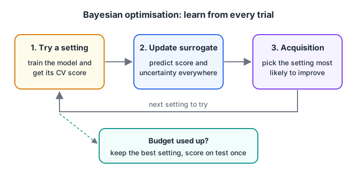
Each expensive evaluation updates the surrogate. The acquisition function balances trying near the current best (exploit) with trying where the surrogate is unsure (explore).
The rule for picking the next trial is the acquisition function. A common one, expected improvement, favours points that are either predicted to score well or are highly uncertain.
You can watch the idea in plain scikit-learn. Here a Gaussian process is the surrogate, tuning one hyperparameter, the SVM's gamma, with C fixed at 10:
import math
import numpy as np
from sklearn.datasets import make_classification
from sklearn.gaussian_process import GaussianProcessRegressor
from sklearn.gaussian_process.kernels import ConstantKernel, Matern
from sklearn.model_selection import cross_val_score
from sklearn.svm import SVC

X, y = make_classification(n_samples=300, n_features=10, n_informative=4,
                           flip_y=0.08, random_state=7)
def score(log_gamma):                                   # the slow, expensive step
    return cross_val_score(SVC(C=10, gamma=10 ** log_gamma), X, y, cv=5).mean()

grid = np.linspace(-4, 1, 200).reshape(-1, 1)          # log10(gamma) from 0.0001 to 10
tried = [-4.0, -1.5, 1.0]                               # three starting guesses
results = [score(g) for g in tried]
kernel = ConstantKernel() * Matern(length_scale=1.0, length_scale_bounds=(0.2, 10))
for step in range(6):
    gp = GaussianProcessRegressor(kernel=kernel, normalize_y=True, alpha=1e-4)
    mu, sd = gp.fit(np.array(tried).reshape(-1, 1), results).predict(grid, return_std=True)
    z = (mu - max(results)) / (sd + 1e-9)
    cdf = np.array([0.5 * (1 + math.erf(v / math.sqrt(2))) for v in z])
    ei = (mu - max(results)) * cdf + sd * np.exp(-z ** 2 / 2) / math.sqrt(2 * math.pi)
    nxt = float(grid[np.argmax(ei), 0])                 # most promising untried gamma
    tried.append(nxt); results.append(score(nxt))
    print(f"step {step + 1}: try gamma = {10 ** nxt:.4f} -> CV accuracy {results[-1]:.3f}")
print(f"best after {len(tried)} evaluations: gamma = {10 ** tried[int(np.argmax(results))]:.4f}")
After three spread-out guesses, the loop quickly concentrates around gamma ≈ 0.01 to 0.02, where accuracy is highest, and still spends a trial or two checking unexplored regions. Nine evaluations were enough; a fine grid over the same range would need far more.
In real projects you would use a library rather than write this loop. Optuna is a popular open-source choice (it uses a tree-structured Parzen estimator by default, a different surrogate):
import optuna
from sklearn.datasets import make_classification
from sklearn.model_selection import cross_val_score
from sklearn.pipeline import make_pipeline
from sklearn.preprocessing import StandardScaler
from sklearn.svm import SVC

X, y = make_classification(n_samples=400, n_features=10, n_informative=4,
                           flip_y=0.08, random_state=7)

def objective(trial):
    C = trial.suggest_float("C", 1e-2, 1e3, log=True)
    gamma = trial.suggest_float("gamma", 1e-4, 10, log=True)
    model = make_pipeline(StandardScaler(), SVC(C=C, gamma=gamma))
    return cross_val_score(model, X, y, cv=5).mean()

study = optuna.create_study(direction="maximize")
study.optimize(objective, n_trials=40)
print(study.best_params, round(study.best_value, 3))
Install it with pip install optuna on your own machine; it does not run in this page's browser sandbox. The Optuna documentation covers pruning, which stops weak trials early.
A practical tuning workflow
- Get a baseline with default settings and record its CV score.
- Tune only the hyperparameters that matter for that model:
Candgammafor an RBF SVM,alphafor ridge and lasso,n_neighborsfor KNN, depth and learning rate for boosting. - Run a wide random search on log scales, 20 to 60 trials.
- Narrow the ranges around the best region and run a second, smaller search or grid.
- Stop when gains fall inside the CV standard deviation. A 0.2-point gain is usually noise.
- Score the final model once on the test set.
When you need an unbiased estimate of the whole tuning procedure, wrap the search inside an outer cross-validation loop. This is called nested cross-validation, and cross_val_score(search, X, y) does it in one line.
Common hyperparameter tuning mistakes
- Tuning on the test set. The test score then stops being an honest estimate.
- Linear ranges for scale-type values. Trying C = 1, 2, 3 … 10 wastes trials; use 0.01, 0.1, 1, 10, 100.
- Scaling outside the pipeline. Each CV fold must fit its own scaler, or validation rows leak into training.
- Huge grids before a baseline. Most of the gain usually comes from one or two hyperparameters.
- Chasing tiny CV gains. Differences smaller than the fold-to-fold spread are not real.
If you want to practise building tuning workflows on real datasets with feedback, the Indore machine learning batch at Debugshala covers model selection end to end. To check your understanding quickly, practise model-tuning MCQs on Debugshala Test.
Key takeaways
- Parameters are learned during training; hyperparameters are set before it and tuned with cross-validation.
- Grid search is exhaustive but its cost multiplies with every hyperparameter you add.
- Random search over log-scale ranges finds good settings with a fixed, smaller budget.
- Bayesian search uses a surrogate model and an acquisition function to choose each next trial; it shines when each fit is slow.
- Keep the test set out of the search and treat gains within the CV spread as noise.
FAQ
What is the difference between a parameter and a hyperparameter?
A parameter is learned from data during training, such as a regression coefficient or a neural network weight. A hyperparameter is set before training and controls how learning happens, such as tree depth, the regularization strength alpha or the learning rate. Hyperparameters are chosen by searching with cross-validation.
Should I use grid search or random search?
Use random search first in most cases. With the same number of trials it explores more values of the hyperparameters that matter, and you control the budget directly. Switch to a small grid search afterwards if you want to check a narrow region around the best result in detail.
What is the best hyperparameter tuning method?
No single method is best for every case. Random search is a strong, simple default. Bayesian optimisation, for example with Optuna, needs fewer trials when each model takes minutes or hours to train. Grid search suits small spaces with two or three hyperparameters and a handful of values each.
How many trials does random search need?
For most tabular models, 20 to 60 random trials over sensible log-scale ranges get close to the best achievable score. Add trials when you tune many hyperparameters or when the CV score is still improving clearly. Stop once improvements are smaller than the standard deviation across folds.
Does Debugshala teach hyperparameter tuning in Indore?
Yes. Hyperparameter tuning with cross-validation is practised in Debugshala's Machine Learning course at the Old Palasia campus in Indore. Classes are offline and taught in English and Hindi, and fresh graduates, non-IT learners and people with a year gap can join. A free demo class is available before you pay.
From the team behind this site
Go further with the Data Science & AI Course at Debugshala
These tutorials are written by Debugshala, a training and placement institute at Old Palasia, Indore. The classroom course adds live mentoring, real projects and interview preparation.
- Offline classes at Old Palasia, Indore
- Free demo class before you pay
- Non-IT, fresher and year-gap friendly
- Placement assistance
700+ students placed · 200+ hiring partners · 4.9★ Google rating
