

Gradient Boosting and XGBoost Explained with Python Code
Gradient boosting explained step by step: residual-fitting trees, learning rate, early stopping, HistGradientBoosting, and what XGBoost adds on top.
A tailor in Indore's Cloth Market is stitching you a kurta. The first cut comes from your rough size, so it is close but loose at the shoulders and long at the sleeves.
At the first fitting the tailor pins only what is still wrong. At the second fitting there is less to fix, so the pins are smaller. After a few rounds, the kurta fits.
The tailor never starts again from scratch. Each fitting corrects the leftover error, and each correction is deliberately modest.
What is gradient boosting?
Map the fittings to machine learning:
- The first rough cut is the initial prediction, often just the average of the target.
- Whatever still doesn't fit is the residual, the gap between the truth and the current prediction.
- Each fitting is a small decision tree trained on those residuals.
- Pinning only part of the gap is the learning rate.
- The finished kurta is the sum of all the corrections.
Gradient boosting is a supervised ensemble learning method that builds decision trees sequentially, training each new tree to predict the remaining errors (the negative gradient of the loss) of the trees before it, and adds the trees' scaled outputs to form the final prediction.
A random forest grows deep trees independently and averages them to cut variance. Boosting grows shallow trees in sequence to cut bias. That is why boosting often wins on tabular data, and why it overfits more easily. The code here targets scikit-learn 1.7 and XGBoost 2.x or later.
Quick check
In gradient boosting for regression, what does each new tree learn to predict?
Each tree fits the remaining errors, the negative gradient of squared loss, and its scaled output is added to the running prediction.
How does gradient boosting work step by step?
For a regression problem with squared error, the algorithm is:
- Start with a constant prediction for every row: the mean of the target.
- Compute each row's residual: actual minus predicted.
- Fit a small tree (depth 2 to 6) that predicts those residuals from the features.
- Update every prediction: add the learning rate times the tree's output.
- Repeat steps 2 to 4 for the chosen number of rounds.
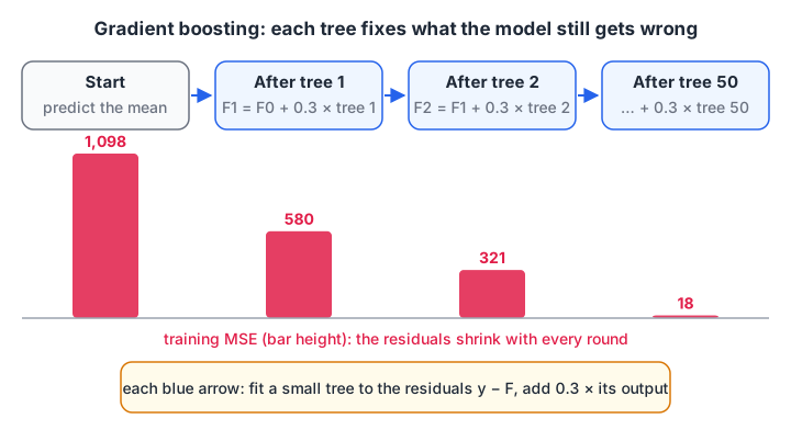
Each tree learns only what the model so far still gets wrong. The learning rate shrinks every correction before it is added.
Here is the whole loop, written by hand, for a lassi stall whose sales rise faster as afternoons get hotter:
import numpy as np
from sklearn.tree import DecisionTreeRegressor
from sklearn.ensemble import GradientBoostingRegressor

# Daily lassi sales at a stall vs afternoon temperature (deg C)
rng = np.random.default_rng(0)
temp = np.sort(rng.uniform(18, 44, 120)).reshape(-1, 1)
sales = 40 + 0.15 * (temp.ravel() - 18) ** 2 + rng.normal(0, 8, 120)

lr, rounds = 0.3, 50
pred = np.full(len(sales), sales.mean())          # round 0: predict the average for everyone
trees = []
for m in range(1, rounds + 1):
    residual = sales - pred                       # what the model still gets wrong
    tree = DecisionTreeRegressor(max_depth=2).fit(temp, residual)
    pred += lr * tree.predict(temp)               # take a small step towards fixing it
    trees.append(tree)
    if m in (1, 2, 5, 10, 50):
        print(f"after {m:2d} trees: training MSE = {np.mean((sales - pred) ** 2):7.1f}")

sk = GradientBoostingRegressor(n_estimators=rounds, learning_rate=lr, max_depth=2).fit(temp, sales)
print("sklearn GradientBoostingRegressor MSE  =", round(np.mean((sales - sk.predict(temp)) ** 2), 1))
print("starting MSE (just the mean)         =", round(sales.var(), 1))
The plain average leaves a training MSE of about 1,098. One small tree brings it to about 580, and 50 trees bring it to about 18. scikit-learn's GradientBoostingRegressor with the same settings gives the same number, because it runs the same loop.
Notice that 18 is well below the noise built into the data (a variance of 64). The model is starting to memorise noise, which is why you always watch a validation score while boosting, not the training score.
Why is it called "gradient" boosting?
For squared error, the residual is exactly the negative gradient of the loss with respect to the prediction. Fitting a tree to residuals is therefore one step of gradient descent, taken in the space of functions rather than weights.
That view lets the same algorithm work with any differentiable loss. Each tree is fitted to the negative gradient of whichever loss you choose:
| Task | Loss | What each tree fits |
|---|---|---|
| Regression | Squared error | Residual: y − prediction |
| Robust regression | Absolute or Huber error | Sign of the residual, or a clipped residual |
| Binary classification | Log loss | y − predicted probability |
| Multi-class | Multinomial log loss | One residual per class |
| Ranking | Pairwise or listwise losses | Gradients over pairs of items |
For classification the trees work on the log-odds scale, and the final sum passes through a sigmoid to give a probability, just as in logistic regression.
Learning rate, number of trees and early stopping
The learning rate and the number of rounds trade off against each other. A large learning rate learns fast but overshoots; a small one needs many more trees but usually ends with a lower error.
import numpy as np
from sklearn.datasets import make_friedman1
from sklearn.ensemble import GradientBoostingRegressor
from sklearn.model_selection import train_test_split

X, y = make_friedman1(n_samples=400, noise=1.0, random_state=0)
Xtr, Xva, ytr, yva = train_test_split(X, y, test_size=0.3, random_state=0)

print("learning rate | best round | best validation MSE")
for lr in [1.0, 0.3, 0.1]:
    gb = GradientBoostingRegressor(learning_rate=lr, n_estimators=300, max_depth=2,
                                   random_state=0).fit(Xtr, ytr)
    val_mse = [np.mean((yva - p) ** 2) for p in gb.staged_predict(Xva)]   # error after each round
    best = int(np.argmin(val_mse))
    print(f"{lr:13} | {best + 1:10d} | {val_mse[best]:.2f}")
staged_predict returns the model's predictions after each round, which lets you find the best round without retraining. With a learning rate of 1.0 the validation error bottoms out after only about 8 trees, at an MSE of about 10.
At 0.1 it keeps improving for almost all 300 rounds and reaches about 3.2. Smaller steps take longer but find a better fit.
Picking the round count by hand is tedious, so libraries offer early stopping: hold out part of the training data, track its loss after every round, and stop when it hasn't improved for a set number of rounds.
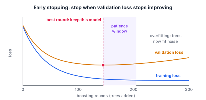
Training loss always falls. Validation loss turns back up once the trees start fitting noise; early stopping keeps the model from around that point.
HistGradientBoosting in scikit-learn
HistGradientBoostingClassifier bins every feature into at most 255 buckets before training, which makes each split search far cheaper. It also handles missing values natively and supports early stopping out of the box.
from sklearn.datasets import make_classification
from sklearn.ensemble import HistGradientBoostingClassifier, RandomForestClassifier
from sklearn.model_selection import train_test_split

X, y = make_classification(n_samples=3000, n_features=20, n_informative=8,
                           flip_y=0.03, random_state=1)
Xtr, Xte, ytr, yte = train_test_split(X, y, test_size=0.25, random_state=0)

hgb = HistGradientBoostingClassifier(max_iter=1000, learning_rate=0.1,
                                     early_stopping=True, validation_fraction=0.15,
                                     n_iter_no_change=20, random_state=0).fit(Xtr, ytr)
print("boosting rounds allowed :", 1000)
print("rounds actually used    :", hgb.n_iter_)
print(f"boosting test accuracy  : {hgb.score(Xte, yte):.3f}")

rf = RandomForestClassifier(n_estimators=60, random_state=0).fit(Xtr, ytr)
print(f"random forest accuracy  : {rf.score(Xte, yte):.3f}")
Allowed up to 1,000 rounds, the model stopped after about 95 because its internal validation loss had stopped improving. It scores about 0.96 on the test set, slightly ahead of a random forest, which is a typical result on clean tabular data.
Quick check
You lower the learning rate from 0.3 to 0.03. What usually happens?
Smaller steps need more rounds to reach a good fit but tend to generalise a little better.
What is XGBoost and how is it different?
XGBoost (eXtreme Gradient Boosting) is an open-source library that implements gradient boosting with a regularised objective, second-order gradient information and heavy engineering for speed. It became famous for winning tabular data competitions, and it remains a standard tool in industry.
What XGBoost adds over the plain algorithm:
- Regularisation in the objective. Penalties on the number of leaves (
gamma) and leaf weights (reg_lambda,reg_alpha) discourage overly complex trees. - Second-order steps. It uses both the gradient and the curvature (Hessian) of the loss, which picks better leaf values.
- Missing-value handling. Each split learns a default direction for missing values.
- Row and column subsampling.
subsampleandcolsample_bytreeadd randomness that reduces overfitting. - Speed. Histogram-based splits, multi-core training and optional GPU training with
device="cuda".
XGBoost isn't available in the browser runner, so this block is for your own machine after pip install xgboost:
import xgboost as xgb
from sklearn.datasets import make_classification
from sklearn.model_selection import train_test_split

X, y = make_classification(n_samples=20000, n_features=30, n_informative=10, random_state=0)
X_train, X_val, y_train, y_val = train_test_split(X, y, test_size=0.2, random_state=0)

model = xgb.XGBClassifier(
    n_estimators=2000,          # an upper limit; early stopping picks the real number
    learning_rate=0.05,
    max_depth=6,
    subsample=0.8,
    colsample_bytree=0.8,
    reg_lambda=1.0,
    tree_method="hist",
    eval_metric="logloss",
    early_stopping_rounds=50,
)
model.fit(X_train, y_train, eval_set=[(X_val, y_val)], verbose=False)
print("best round:", model.best_iteration)
print("validation accuracy:", model.score(X_val, y_val))   # uses the best round
XGBoost vs LightGBM vs CatBoost vs scikit-learn
| Library | Distinctive idea | Good fit |
|---|---|---|
scikit-learn HistGradientBoosting* |
Histogram boosting, no extra install | First model, medium data, pipelines |
| XGBoost | Regularised objective, mature GPU support | General tabular work, large data |
| LightGBM | Leaf-wise tree growth, very fast on large data | Millions of rows, many features |
| CatBoost | Built-in handling of categorical columns | Data with many text categories |
Once tuned, the four usually score within a whisker of each other, so choose by data size and categorical columns.
Common gradient boosting mistakes
- Judging by training error. Boosting can drive it close to zero. Use a validation set or early stopping.
- A high learning rate with many trees. Lower the rate and let early stopping pick the rounds.
- Deep trees by habit. Boosting works best with shallow trees, often depth 3 to 6.
- Early stopping on the test set. That leaks the test set into training. Use a separate validation split.
- Tuning everything at once. Fix the learning rate, find the rounds, then tune depth and subsampling with hyperparameter tuning.
Boosting rewards careful validation habits, which are easier to build with a mentor reviewing your experiments in a trainer-led machine learning course in Indore. The next tutorial, ensemble learning, puts bagging, boosting and stacking side by side. To check yourself first, practise boosting MCQs on Debugshala Test.
Key takeaways
- Gradient boosting adds shallow trees one at a time, each correcting the errors of the model so far.
- The residuals are the negative gradient of the loss, so any differentiable loss works.
- Learning rate and rounds trade off; use a small rate and early stopping on a validation split.
- XGBoost adds regularisation, second-order steps and speed; LightGBM, CatBoost and scikit-learn's HistGradientBoosting are close alternatives.
- Boosting reduces bias, forests reduce variance; boosting needs more careful validation.
FAQ
What is the difference between random forest and gradient boosting?
A random forest trains deep trees independently on random samples and averages them, which mainly reduces variance. Gradient boosting trains shallow trees one after another, each correcting the last, which mainly reduces bias. Boosting is often more accurate on tabular data after tuning, while a forest is easier to train well with default settings.
Is XGBoost the same as gradient boosting?
XGBoost is one implementation of gradient boosting, not a different algorithm. It adds a regularised objective, second-order gradient steps, built-in missing-value handling and fast histogram and GPU training. The core idea of adding trees that correct earlier errors is the same as in scikit-learn's GradientBoostingClassifier.
What is a good learning rate for gradient boosting?
A learning rate between 0.03 and 0.1 is a common starting range. Pair it with a generous upper limit on the number of trees and early stopping on a validation split, so the library picks the round count for you. Higher rates train faster but usually end with a slightly worse validation score.
Does gradient boosting need feature scaling?
No. Like all tree-based models, gradient boosting splits on thresholds within one feature at a time, so scaling a feature doesn't change the result. You still need to encode categories, unless you use a library with native categorical support such as CatBoost or the categorical_features option in scikit-learn's HistGradientBoosting.
Can I learn XGBoost and boosting at Debugshala in Indore?
Yes. Gradient boosting and the other ensemble methods are covered in Debugshala's Machine Learning course, taught offline at 204-208 C.S. Naidu Arcade, Old Palasia, Indore. Classes are in English and Hindi, fresh graduates and non-IT learners are welcome, and you can attend a free demo class first.
From the team behind this site
Go further with the Data Science & AI Course at Debugshala
These tutorials are written by Debugshala, a training and placement institute at Old Palasia, Indore. The classroom course adds live mentoring, real projects and interview preparation.
- Offline classes at Old Palasia, Indore
- Free demo class before you pay
- Non-IT, fresher and year-gap friendly
- Placement assistance
700+ students placed · 200+ hiring partners · 4.9★ Google rating
