

Hierarchical Clustering Explained: Dendrograms and Linkage
Hierarchical clustering explained: how agglomerative merging works, reading a dendrogram, single vs complete vs average vs Ward linkage, and cutting the tree.
Your cousin's wedding is in two weeks, and you've been handed the guest list for seating. Nobody gave you a number of tables.
So you begin with the obvious pairs: siblings sit together, then each pair of siblings joins their parents, then families from the same mohalla join up, and finally everything rolls up into the bride's side and the groom's side.
When you're done, you have more than one seating plan. You have the whole family tree of groupings. If the hall has two big tables, cut the tree near the top. If it has ten, cut it lower down. The tree comes first; the number of tables is a decision you make by looking at it.
What is hierarchical clustering?
Map the seating job to machine learning:
- Each guest is a data point, with no labels.
- "How closely related" two guests are is the distance between points.
- Seating the two closest groups together is one merge.
- The record of all merges, with the distance at which each happened, is the dendrogram.
- Choosing how many tables to use is cutting the dendrogram.
Hierarchical clustering is an unsupervised learning method that builds a nested hierarchy of clusters, either by repeatedly merging the closest clusters (agglomerative) or by repeatedly splitting clusters (divisive), and shows the result as a tree called a dendrogram.
There are two directions:
| Agglomerative (bottom-up) | Divisive (top-down) | |
|---|---|---|
| Starts with | Every point as its own cluster | All points in one cluster |
| Each step | Merges the two closest clusters | Splits one cluster in two |
| In scikit-learn and SciPy | Yes: AgglomerativeClustering, scipy.cluster.hierarchy |
Not directly; BisectingKMeans is a related idea |
| Used in practice | Almost always | Rarely |
The rest of this tutorial is about the agglomerative version. It follows k-means clustering, which needs k up front; hierarchical clustering lets you postpone that choice. The code targets SciPy and scikit-learn 1.7.
How does agglomerative clustering work?
- Treat each of the n points as its own cluster.
- Compute the distance between every pair of clusters.
- Merge the closest pair into one cluster and record the distance at which they merged.
- Update the distances from the new cluster to every other cluster, using the chosen linkage rule.
- Repeat steps 3 and 4 until a single cluster contains all points (n − 1 merges in total).
SciPy's linkage returns those merges as a table, one row per merge. Here are six points, A to F, on a map:
import numpy as np
from scipy.cluster.hierarchy import fcluster, linkage

names = ["A", "B", "C", "D", "E", "F"]
X = np.array([[1.0, 1.0], [1.4, 1.3], [5.0, 1.2], [5.6, 1.0], [5.2, 4.8], [3.0, 3.0]])

Z = linkage(X, method="average")            # each row of Z is one merge
clusters = {i: names[i] for i in range(len(names))}
for step, (a, b, dist, size) in enumerate(Z, start=1):
    new = clusters[int(a)] + clusters[int(b)]
    clusters[len(names) + step - 1] = new
    print(f"merge {step}: {clusters[int(a)]:>4} + {clusters[int(b)]:<4} at distance {dist:.2f} -> {new} ({int(size)} points)")

for k in (2, 3):
    labels = fcluster(Z, t=k, criterion="maxclust")
    print(f"cut into {k} clusters:", " ".join(f"{n}={l}" for n, l in zip(names, labels)))
A and B merge first, at a distance of 0.50, then C and D at 0.63. F joins A and B at about 2.6, E joins C and D at about 3.7, and the two groups merge last at about 4.0.
fcluster cuts the tree: asking for 2 clusters gives (A, B, F) and (C, D, E); asking for 3 splits E off on its own.
How do you read a dendrogram?
A dendrogram draws each merge as a horizontal bar joining two branches. The height of the bar is the distance at which those clusters merged.
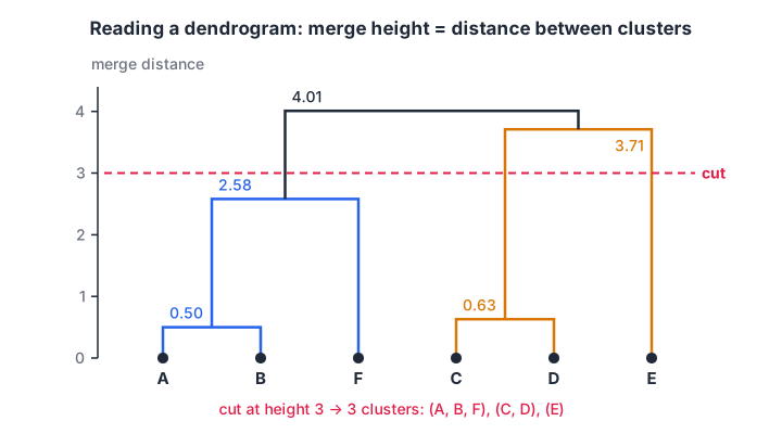
Short bars near the bottom join very similar points. A horizontal cut at height 3 crosses three vertical lines, so it gives three clusters: (A, B, F), (C, D) and (E).
Three rules make dendrograms easy to read:
- Height matters, left-to-right order doesn't. Branches can be swapped without changing the meaning.
- Long vertical gaps signal real structure. If clusters merge low and then nothing happens for a long stretch, that stretch is a natural place to cut.
- The number of vertical lines your cut crosses is the number of clusters.
Quick check
In agglomerative clustering, what does the height of a merge in a dendrogram show?
The y-axis of a dendrogram is merge distance. Low merges join similar points.
Linkage methods: single, complete, average and Ward
Once a cluster holds more than one point, "the distance between two clusters" needs a definition. That definition is the linkage.
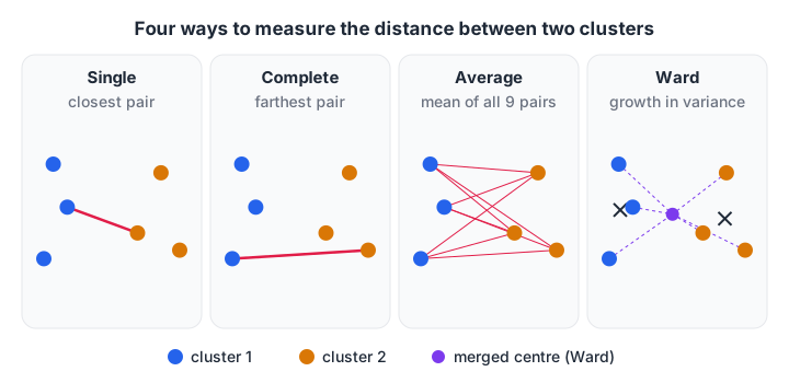
The same two clusters can be close under single linkage and far apart under complete linkage.
| Linkage | Distance between clusters | Tends to produce | Watch out for |
|---|---|---|---|
| Single | Closest pair of points | Long, chain-like clusters; follows curves | Chaining: a thin bridge merges two groups |
| Complete | Farthest pair of points | Compact clusters of similar diameter | Sensitive to outliers |
| Average | Mean of all pairwise distances | A balance between single and complete | Middle-of-the-road on odd shapes |
| Ward | Increase in total within-cluster variance | Compact, similar-sized clusters, like k-means | Euclidean distance only |
The choice changes results dramatically, as two small datasets show:
import numpy as np
from sklearn.cluster import AgglomerativeClustering
from sklearn.datasets import make_blobs, make_moons
from sklearn.metrics import adjusted_rand_score

rng = np.random.default_rng(0)
blobs, yb = make_blobs(n_samples=300, centers=[[0, 0], [6, 0]], cluster_std=1.0, random_state=1)
bridge = np.column_stack([np.linspace(1.5, 4.5, 15), rng.normal(0, 0.1, 15)])   # a thin chain of points
X_bridge = np.vstack([blobs, bridge])
y_bridge = np.concatenate([yb, (bridge[:, 0] > 3).astype(int)])
X_moons, y_moons = make_moons(n_samples=300, noise=0.05, random_state=0)

print("linkage  | blobs + bridge | two moons   (adjusted Rand index, 1 = perfect)")
for method in ["single", "complete", "average", "ward"]:
    scores = []
    for X, y in [(X_bridge, y_bridge), (X_moons, y_moons)]:
        labels = AgglomerativeClustering(n_clusters=2, linkage=method).fit_predict(X)
        scores.append(adjusted_rand_score(y, labels))
    print(f"{method:8s} | {scores[0]:14.2f} | {scores[1]:.2f}")
The adjusted Rand index compares found clusters with the true groups (1 is a perfect match, 0 is chance). On two blobs joined by a thin bridge of points, single linkage scores 0.00: it walks across the bridge and merges both blobs early, leaving a stray point as the "second cluster".
Complete and Ward handle it well. On two interlocking moons the picture flips. Single linkage follows each curve and scores 1.00, while Ward and complete cut the moons with a straight line.
No linkage is best everywhere. Start with Ward for blob-shaped business data, and try single or average when clusters may be curved or elongated.
Quick check
Two well-separated blobs are joined by a thin line of points. Which linkage is most likely to merge the blobs too early?
Single linkage uses the closest pair of points, so a chain of nearby points links the blobs. This is called chaining.
How do you choose the number of clusters?
You can cut the tree in two ways: ask for a fixed number of clusters, or set a distance threshold and let the number of clusters follow. scikit-learn supports both through AgglomerativeClustering.
import numpy as np
from sklearn.cluster import AgglomerativeClustering
from sklearn.datasets import make_blobs
from sklearn.preprocessing import StandardScaler

X, _ = make_blobs(n_samples=200, centers=4, cluster_std=0.8, random_state=3)
X = StandardScaler().fit_transform(X)

print("distance threshold | clusters found")
for t in [0.5, 1, 3, 6, 10, 20, 30]:
    model = AgglomerativeClustering(n_clusters=None, distance_threshold=t, linkage="ward")
    print(f"{t:18} | {model.fit(X).n_clusters_}")

model = AgglomerativeClustering(n_clusters=None, distance_threshold=0, linkage="ward").fit(X)
heights = np.sort(model.distances_)[::-1]
print("five tallest merge heights:", heights[:5].round(2))
A low threshold leaves many small clusters, and a high one leaves one. Between 3 and 6 the answer holds steady at 4, and the merge heights explain why: the fourth-tallest merge is at about 1.4, the third-tallest jumps to about 8.1.
That big gap is the long vertical stretch in the dendrogram, and cutting inside it gives the four groups.
To draw the dendrogram on your own machine, use SciPy with matplotlib:
import matplotlib.pyplot as plt
from scipy.cluster.hierarchy import dendrogram, linkage
from sklearn.datasets import make_blobs
from sklearn.preprocessing import StandardScaler

X, _ = make_blobs(n_samples=200, centers=4, cluster_std=0.8, random_state=3)
Z = linkage(StandardScaler().fit_transform(X), method="ward")

plt.figure(figsize=(10, 4))
dendrogram(Z, truncate_mode="lastp", p=20)   # show only the last 20 merges
plt.axhline(y=4, linestyle="--")             # a candidate cut
plt.ylabel("merge distance")
plt.tight_layout()
plt.show()
Hierarchical clustering vs k-means
| Hierarchical (agglomerative) | K-means | |
|---|---|---|
| Number of clusters | Chosen after building the tree | Must be chosen before running |
| Output | Full tree plus any flat cut | One flat set of k clusters |
| Deterministic | Yes, for a given linkage | Depends on starting centroids |
| Cluster shapes | Depends on linkage; single follows curves | Round blobs |
| Memory and time | About n² distances; slow beyond tens of thousands of rows | Scales to millions of rows |
| Best for | Small data, exploring structure, taxonomies | Large data, round groups |
The n² cost is the main practical limit: 20,000 rows already means about 200 million pairwise distances. For bigger data, cluster a sample hierarchically to choose k, then run k-means on everything. If clusters have odd shapes and noise, DBSCAN, the next tutorial, is often the better fit.
Common hierarchical clustering mistakes
- Not scaling features. As with every distance-based method, the largest unit dominates; see data preprocessing: scaling and encoding.
- Using Ward with non-Euclidean distances. Ward is defined for Euclidean distance only; use average or complete linkage for others.
- Running it on 100,000 rows. Memory grows with n²; sample first.
- Reading meaning into left-right order. Only heights carry information.
- Defaulting to one linkage. Compare at least two, because results can differ completely.
Reading dendrograms well comes with practice on real data, the kind of exercise done in the Old Palasia machine learning course. For quick revision, attempt linkage and dendrogram questions on Debugshala Test.
Key takeaways
- Agglomerative clustering starts with single points and merges the closest clusters until one remains.
- The dendrogram records every merge; cutting it at a height gives flat clusters.
- Linkage defines cluster distance: single follows chains, complete and Ward give compact groups, average sits between.
- Look for a long vertical gap in the dendrogram to choose the number of clusters.
- It costs about n² memory, so it suits small and medium datasets.
FAQ
What is a dendrogram in hierarchical clustering?
A dendrogram is a tree diagram that shows the order and distance of every merge in hierarchical clustering. Points sit along the bottom, and each horizontal bar joins two clusters at the height equal to their distance. Cutting the tree with a horizontal line gives a flat set of clusters.
What is the difference between agglomerative and divisive clustering?
Agglomerative clustering works bottom-up: each point starts alone and the closest clusters merge step by step. Divisive clustering works top-down: all points start in one cluster, which is split repeatedly. Agglomerative is far more common and is what scikit-learn's AgglomerativeClustering and SciPy's linkage implement.
Which linkage method is best?
No single linkage is best. Ward is a strong default for compact, similar-sized groups in Euclidean space. Single linkage finds curved or elongated clusters but suffers from chaining. Complete and average linkage sit in between. Compare a couple of options on your data, using silhouette scores or domain knowledge.
Is hierarchical clustering better than k-means?
It is better when you don't know the number of clusters, want to see nested structure, or have a small dataset. K-means is better for large datasets because it scales to millions of rows. A common workflow uses hierarchical clustering on a sample to choose k, then k-means on the full data.
Where can I practise clustering with a mentor in Indore?
Debugshala's Machine Learning course in Indore covers hierarchical clustering, k-means and DBSCAN with hands-on exercises at the Old Palasia campus. It is taught offline in English and Hindi and accepts learners without an IT background. You can join a free demo class before deciding; call +91-8982385539.
From the team behind this site
Go further with the Data Science & AI Course at Debugshala
These tutorials are written by Debugshala, a training and placement institute at Old Palasia, Indore. The classroom course adds live mentoring, real projects and interview preparation.
- Offline classes at Old Palasia, Indore
- Free demo class before you pay
- Non-IT, fresher and year-gap friendly
- Placement assistance
700+ students placed · 200+ hiring partners · 4.9★ Google rating
