

DBSCAN Clustering Explained: eps, min_samples and Noise
DBSCAN clustering explained: core, border and noise points, choosing eps with a k-distance plot, DBSCAN vs k-means on curved data, and when to use HDBSCAN.
Picture a drone photo of Sarafa Bazaar at 10 pm. You can see crowds immediately: a thick knot of people around the garadu stall, another around the bhutte ka kees counter, and a long, curving stream along the lane. Here and there a few people stand alone.
How did you spot the crowds? Not by guessing that there were three. You looked for places where people stand close to many others and followed those dense patches, even around a bend. The loners belonged to no crowd.
What is DBSCAN clustering?
Map the drone photo to machine learning:
- Each person is a data point.
- "Standing close" means within a radius eps of each other.
- Someone with at least min_samples people (counting themselves) within eps is a core point: the heart of a crowd.
- Someone near a core point but without enough neighbours of their own is a border point: the edge of a crowd.
- Someone near nobody dense is noise, labelled −1.
- A crowd is a cluster: core points chained together by being within eps of each other, plus their border points.
DBSCAN is an unsupervised, density-based clustering algorithm that groups points lying in dense regions, defined by a radius eps and a minimum neighbour count min_samples, into clusters of arbitrary shape and labels points in low-density regions as noise.
K-means and hierarchical clustering put every point in some cluster. DBSCAN can say "this point belongs nowhere". The code targets scikit-learn 1.7.
Quick check
Which situation favours HDBSCAN over DBSCAN?
HDBSCAN effectively tries every eps and keeps stable clusters, so it copes with dense and sparse clusters together.
Core, border and noise points
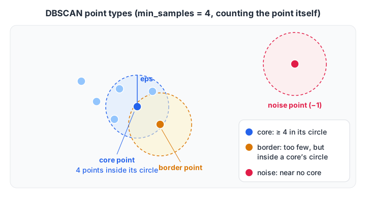
With min_samples = 4, the blue point has 4 points (itself included) inside its eps circle, so it is a core point. The amber point is reachable from a core point but has only one neighbour, so it is a border point. The rose point is noise.
Here is a tiny version of the drone photo, with 13 people:
import numpy as np
from sklearn.cluster import DBSCAN

# positions (metres) of 13 people in a drone photo of a market street
X = np.array([[1, 1], [1.5, 1.2], [1.2, 1.8], [2, 1.5], [1.6, 0.6],     # group near a chaat stall
              [8, 8], [8.5, 8.4], [8.2, 7.6], [7.6, 8.1],                # group at a juice counter
              [2.9, 1.9],                                                # someone at the edge of group 1
              [5, 5], [12, 2], [4.5, 9]])                                # lone walkers

db = DBSCAN(eps=1.0, min_samples=4).fit(X)
core = np.zeros(len(X), dtype=bool)
core[db.core_sample_indices_] = True
for i, (label, is_core) in enumerate(zip(db.labels_, core)):
    kind = "core" if is_core else ("noise" if label == -1 else "border")
    print(f"person {i:2d} at {X[i].tolist()}: cluster {label:2d} ({kind})")
The five people around the chaat stall and the four at the juice counter are all core points. Person 9 stands within 1 metre of a core point but has only one neighbour, so it joins cluster 0 as a border point.
The three lone walkers get the label −1. Notice that you never said there were two clusters; DBSCAN found that from the density.
Quick check
In DBSCAN with min_samples = 5, a point has 3 points (itself included) within eps, one of which is a core point. What is it?
It lacks enough neighbours to be core, but it lies inside a core point's neighbourhood, so it joins that cluster as a border point.
How does the DBSCAN algorithm work?
- For every point, find all points within distance eps (its neighbourhood).
- Mark points whose neighbourhood holds at least min_samples points as core points.
- Pick an unvisited core point and start a new cluster.
- Add every point in its neighbourhood to the cluster. Whenever an added point is itself a core point, add its neighbourhood too, and keep expanding.
- When the cluster stops growing, move on to the next unvisited core point and repeat from step 3.
- Any point never reached from a core point is noise.
Because clusters grow by hopping from core point to core point, they can snake around corners.
DBSCAN vs k-means on curved clusters
K-means draws straight boundaries between centres, so two interlocking half-moons defeat it, and it can't set outliers aside.
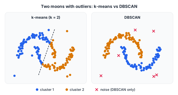
Same data, two algorithms. K-means cuts both moons in half. DBSCAN follows each moon and leaves the scattered points unlabelled.
import numpy as np
from sklearn.cluster import DBSCAN, KMeans
from sklearn.datasets import make_moons
from sklearn.metrics import adjusted_rand_score

X, y = make_moons(n_samples=400, noise=0.06, random_state=0)
rng = np.random.default_rng(0)
X = np.vstack([X, rng.uniform([-1.5, -1], [2.5, 1.5], (20, 2))])   # 20 scattered outliers
y = np.concatenate([y, np.full(20, -1)])

km = KMeans(n_clusters=2, n_init=10, random_state=0).fit_predict(X)
db = DBSCAN(eps=0.2, min_samples=5).fit_predict(X)
moons = y != -1
print(f"k-means: ARI on the moons {adjusted_rand_score(y[moons], km[moons]):.2f}, "
      f"outliers flagged: 0 of 20 (k-means assigns every point)")
print(f"DBSCAN : ARI on the moons {adjusted_rand_score(y[moons], db[moons]):.2f}, "
      f"clusters found: {db.max() + 1}, noise points: {(db == -1).sum()} "
      f"({(db[~moons] == -1).sum()} of them real outliers)")
The adjusted Rand index (1 means a perfect match with the true groups) is about 0.25 for k-means and 1.00 for DBSCAN on the moon points. DBSCAN also marked 12 points as noise, all of them genuine outliers.
The other 8 outliers happened to land close to a moon and were absorbed, which is the honest behaviour of a density method: a point in a dense spot looks normal.
That built-in noise label makes DBSCAN a handy first tool for anomaly detection, such as spotting unusual transactions or sensor readings.
How do you choose eps and min_samples?
These two settings decide everything, so choose them deliberately.
min_samples first. A common rule of thumb is twice the number of features, with a minimum of 3 or 4. Larger values make DBSCAN stricter: fewer core points, more noise and smoother clusters. Raise it for noisy data.
eps next, using a k-distance plot:
- Set k = min_samples.
- For every point, compute the distance to its k-th nearest neighbour (scikit-learn counts the point itself as the first).
- Sort those distances and plot them.
- Look for the "knee", where the curve turns sharply upward. Points left of the knee sit inside clusters; points right of it are outliers. The distance at the knee is a good eps.
import numpy as np
from sklearn.cluster import DBSCAN
from sklearn.datasets import make_blobs
from sklearn.neighbors import NearestNeighbors
from sklearn.preprocessing import StandardScaler

X, _ = make_blobs(n_samples=500, centers=3, cluster_std=0.6, random_state=6)
X = np.vstack([X, np.random.default_rng(1).uniform(X.min(0) - 2, X.max(0) + 2, (25, 2))])   # 25 outliers
X = StandardScaler().fit_transform(X)
min_samples = 4                                      # 2 x number of features

dist, _ = NearestNeighbors(n_neighbors=min_samples).fit(X).kneighbors(X)
k_dist = np.sort(dist[:, -1])                       # distance to the 4th nearest point (itself included)
print("k-distance percentiles (50, 90, 95, 98, 99):",
      np.percentile(k_dist, [50, 90, 95, 98, 99]).round(3))

print("  eps | clusters | noise points")
for eps in [0.03, 0.08, 0.15, 0.3, 0.8]:
    labels = DBSCAN(eps=eps, min_samples=min_samples).fit_predict(X)
    print(f"{eps:5} | {labels.max() + 1:8d} | {(labels == -1).sum()}")
The 4th-neighbour distance is about 0.03 for the median point and 0.13 at the 95th percentile, then it jumps to about 0.6 at the 98th. That jump is the knee, and it lines up with the roughly 5% of rows that are outliers.
An eps below the knee (0.03) shatters the data into 15 fragments with 157 noise points. Anything from 0.08 to 0.3 finds the 3 real clusters, with 18 to 34 noise points. An eps of 0.8, past the knee, swallows all the outliers into clusters.
Always scale features before DBSCAN; eps is a single radius applied to every feature, so a column measured in thousands would dominate it. Data preprocessing: scaling and encoding covers the options.
Quick check
Your DBSCAN run labels 70% of points as -1. What is the most likely fix?
Too much noise means neighbourhoods are too strict. A larger radius or a lower neighbour count creates more core points.
When DBSCAN struggles: varying density and HDBSCAN
One eps can't fit tight and spread-out clusters at once: a small eps breaks the loose cluster into noise, and a large one merges the tight clusters with their neighbours.
HDBSCAN (hierarchical DBSCAN) runs DBSCAN across all values of eps at once, builds a tree of clusters, and keeps the ones that persist the longest. You give it a min_cluster_size instead of eps. scikit-learn has included HDBSCAN since version 1.3.
import numpy as np
from sklearn.cluster import DBSCAN, HDBSCAN
from sklearn.datasets import make_blobs
from sklearn.metrics import adjusted_rand_score

# a tight, a medium and a very loose cluster: three different densities
X, y = make_blobs(n_samples=[150, 150, 150], centers=[[0, 0], [3, 3], [9, 0]],
                  cluster_std=[0.3, 0.8, 2.0], random_state=4)

for eps in [0.3, 0.8, 1.2]:
    labels = DBSCAN(eps=eps, min_samples=8).fit_predict(X)
    print(f"DBSCAN eps={eps}: clusters {labels.max() + 1}, noise {(labels == -1).sum():3d}, "
          f"ARI {adjusted_rand_score(y, labels):.2f}")

labels = HDBSCAN(min_cluster_size=20, copy=True).fit_predict(X)
print(f"HDBSCAN        : clusters {labels.max() + 1}, noise {(labels == -1).sum():3d}, "
      f"ARI {adjusted_rand_score(y, labels):.2f}")
No single eps recovers the three clusters here. With eps = 0.3 and 0.8, DBSCAN splits the data into 4 clusters and marks many points of the loose cluster as noise; with 1.2 it merges the tight and medium clusters into 2. HDBSCAN finds all 3 with no eps at all and the best agreement, an ARI of about 0.89.
Comparing clustering algorithms
| K-means | Hierarchical | DBSCAN | HDBSCAN | |
|---|---|---|---|---|
| Number of clusters | You choose k | You cut the tree | Found from density | Found from density |
| Cluster shapes | Round blobs | Depends on linkage | Any shape | Any shape |
| Handles noise | No, every point assigned | No | Yes, label −1 | Yes, label −1 |
| Varying density | Poor | Fair | Poor | Good |
| Key settings | k, n_init | Linkage, cut height | eps, min_samples | min_cluster_size |
| Large data | Very fast | Slow (n²) | Fast with spatial indexes in low dimensions | Moderate |
DBSCAN's neighbourhood search is fast in a few dimensions but weakens as features multiply, because distances lose contrast in high dimensions. Reduce the number of features first; PCA and dimensionality reduction, the next tutorial, shows how.
Common DBSCAN mistakes
- Not scaling features. One eps radius covers every feature, so units must match.
- Guessing eps. Use a k-distance plot; small changes in eps can change the result completely.
- Reading label −1 as a cluster. It means noise. Exclude it when counting clusters or profiling them.
- Using DBSCAN on very high-dimensional data. Reduce dimensions first.
- Expecting one eps to fit clusters of different densities. Switch to HDBSCAN or OPTICS.
If you want feedback on a real clustering or outlier project, an offline machine learning course at Debugshala pairs you with a trainer. For self-checks, check your density-clustering skills on Debugshala Test.
Key takeaways
- DBSCAN builds clusters from dense regions and labels sparse points as noise (−1).
- Core points have at least min_samples neighbours within eps; border points sit beside them; everything else is noise.
- It finds any cluster shape and needs no number of clusters.
- Choose min_samples first (about twice the feature count), then eps from the knee of a k-distance plot, on scaled data.
- For clusters of different densities, use HDBSCAN.
FAQ
What is eps in DBSCAN?
eps is the radius of the neighbourhood DBSCAN draws around each point. Points within eps of each other count as neighbours. A small eps produces many small clusters and lots of noise, while a large eps merges clusters together. Choose it from the knee of a k-distance plot on scaled data.
Is DBSCAN better than k-means?
DBSCAN is better when clusters are curved or irregular, when the data contains outliers, or when you don't know how many clusters exist. K-means is better for large datasets of round, similar-sized groups and when every point must belong to a cluster. Many projects try both and compare.
Does DBSCAN need the number of clusters?
No. DBSCAN discovers the number of clusters from the data's density, using only eps and min_samples. That is one of its biggest advantages over k-means. The trade-off is that eps and min_samples must be chosen carefully, because they decide how many clusters appear.
Can DBSCAN be used for outlier detection?
Yes. DBSCAN labels points in low-density regions as noise with the value −1, which makes it a simple, effective outlier detector for low-dimensional data. Points close to a dense area can still be absorbed into a cluster, so combine it with domain checks or dedicated methods like isolation forest for important cases.
Does Debugshala teach DBSCAN and unsupervised learning in Indore?
Yes. DBSCAN, k-means and hierarchical clustering are taught in Debugshala's Machine Learning course at the Old Palasia campus, Indore. Classes are offline in English and Hindi, fresh graduates and non-IT learners can join, and placement assistance is offered. A free demo class lets you try the teaching before you pay.
From the team behind this site
Go further with the Data Science & AI Course at Debugshala
These tutorials are written by Debugshala, a training and placement institute at Old Palasia, Indore. The classroom course adds live mentoring, real projects and interview preparation.
- Offline classes at Old Palasia, Indore
- Free demo class before you pay
- Non-IT, fresher and year-gap friendly
- Placement assistance
700+ students placed · 200+ hiring partners · 4.9★ Google rating
