

Logistic Regression Explained: Sigmoid, Odds and Python Code
Logistic regression explained: how the sigmoid turns a score into a probability, odds ratios, log loss, softmax for many classes and the C parameter in sklearn.
Think of a placement coordinator at an engineering college in Indore before campus interview season. For every final-year student she knows two things: how many hours of mock interviews they practised and their aptitude test score. She wants to know who is likely to clear the first round, so she can give extra coaching to the borderline group.
A yes/no list isn't enough for her. A student with a 51% chance and one with a 98% chance both get "yes", but only one needs help. What she wants is a probability for every student.
Logistic regression gives her exactly that.
What is logistic regression?
Map the coordinator's problem to the terms:
- Practice hours and aptitude score are the features.
- "Cleared" (1) or "not cleared" (0) is the binary target.
- The chance of clearing is the predicted probability, P(y = 1).
- Her cut-off for calling a student "likely to clear" is the decision threshold, 0.5 by default.
Logistic regression is a supervised classification algorithm that models the probability of a class as the sigmoid of a linear combination of the input features, and is fitted by minimising log loss.
Despite the name, it is used for classification, not for predicting numbers. The "regression" part refers to the linear score inside it, which is the same weighted sum you met in linear regression explained. This tutorial targets scikit-learn 1.7.
Why not use linear regression for classification?
You could code the target as 0 and 1 and fit a straight line. Three things go wrong:
- The line predicts values below 0 and above 1, which can't be probabilities.
- A few extreme rows, such as a student with 200 practice hours, tilt the whole line and move the cut-off.
- Squared error is a poor measure for yes/no outcomes; it barely punishes confident wrong answers.
Logistic regression fixes all three by bending the output into an S-shaped curve.
How does the sigmoid function turn a score into a probability?
The model first computes a linear score, often called z or the log-odds:
z = b0 + b1 × hours + b2 × aptitudeThen it applies the sigmoid (logistic) function:
P(cleared) = 1 / (1 + e^(−z))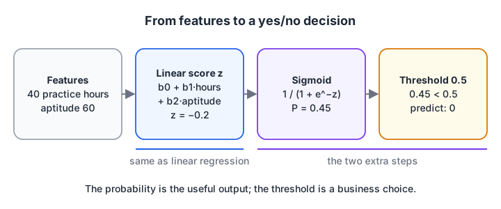
Logistic regression is linear regression with two extra steps at the end: squash the score into 0 to 1, then cut it at a threshold.
import numpy as np

def sigmoid(z):
    return 1 / (1 + np.exp(-z))

scores = np.array([-6, -2, -0.5, 0, 0.5, 2, 6])
for z, p in zip(scores, sigmoid(scores)):
    print(f"score z = {z:5.1f}  ->  probability {p:.3f}")

# the inverse: probability -> odds -> log-odds (back to the score)
p = 0.8
print("p = 0.8 -> odds", round(p / (1 - p), 2), "-> log-odds", round(np.log(p / (1 - p)), 3))
A score of 0 maps to exactly 0.5. Large positive scores approach 1 and large negative ones approach 0, but never cross them.
The inverse is the logit: a probability of 0.8 means odds of 4 to 1 and a log-odds of about 1.39. So the linear part of the model predicts log-odds, and the sigmoid converts log-odds back into probability.
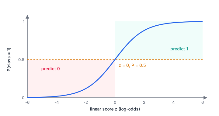
The S-curve is steepest around a score of 0, where the model is least sure. Far from 0, extra evidence changes the probability very little.
Quick check
The linear score z for a customer is 0. What probability does logistic regression give?
The sigmoid of 0 is 1 / (1 + e^0) = 1 / 2 = 0.5.
Logistic regression in Python with scikit-learn
Here are 400 synthetic students. The hidden rule gives better odds for more practice and higher aptitude, with plenty of randomness, as in real life.
import numpy as np
from sklearn.linear_model import LogisticRegression

rng = np.random.default_rng(4)
n = 400
hours = rng.uniform(0, 60, n)                  # hours of mock interviews practised
aptitude = rng.uniform(30, 100, n)             # aptitude test score
z = -7 + 0.08 * hours + 0.06 * aptitude        # hidden "true" log-odds
placed = (rng.random(n) < 1 / (1 + np.exp(-z))).astype(int)
X = np.column_stack([hours, aptitude])

model = LogisticRegression().fit(X, placed)
b0, (b_hours, b_apt) = model.intercept_[0], model.coef_[0]
print(f"log-odds = {b0:.2f} + {b_hours:.3f} x hours + {b_apt:.3f} x aptitude")
print(f"odds ratio per extra hour: {np.exp(b_hours):.3f}")
print(f"odds ratio per 10 extra hours: {np.exp(10 * b_hours):.2f}")

students = np.array([[10, 60], [40, 60], [40, 85]])
for (h, a), p in zip(students, model.predict_proba(students)[:, 1]):
    print(f"{h:2.0f} hours, aptitude {a:.0f}: P(placed) = {p:.2f} -> predict {int(p >= 0.5)}")
predict_proba returns one column per class; column 1 holds P(cleared). predict applies the 0.5 threshold for you. The student with 40 hours and an aptitude of 60 sits at 0.45: a borderline case worth the coordinator's time, which a plain yes/no would hide.
How do you interpret logistic regression coefficients?
Coefficients live on the log-odds scale, which is hard to feel. Exponentiate them to get odds ratios:
- exp(0.069) ≈ 1.07: each extra hour of practice multiplies the odds of clearing by about 1.07, a 7% rise in the odds.
- Ten extra hours multiply the odds by about 2.0, so they double.
- An odds ratio above 1 means the feature raises the chance; below 1 means it lowers it; exactly 1 means no effect.
Odds are not probabilities. Doubling the odds moves a student from 0.09 to about 0.17, but moves a borderline 0.45 student to about 0.62. The effect on probability depends on where on the S-curve you start.
The model recovered coefficients of 0.069 and 0.049 against true values of 0.08 and 0.06. They are a bit smaller partly because of noise and partly because scikit-learn applies L2 regularization by default.
Quick check
A coefficient for "number of complaints" is 0.69. What is the odds ratio for one extra complaint?
exp(0.69) ≈ 2.0, so each extra complaint roughly doubles the odds of the positive class.
Quick check
In scikit-learn, what happens when you decrease C in LogisticRegression?
C is the inverse of regularization strength, so a smaller C means a larger penalty on coefficients.
How is logistic regression trained? Log loss
Logistic regression chooses its coefficients by minimising log loss (also called binary cross-entropy). For each row it takes the predicted probability of the true class and adds −log of it. A confident correct prediction costs almost nothing; a confident wrong one costs a lot.
import numpy as np
from sklearn.metrics import log_loss

y_true = np.array([1, 1, 0, 0, 1])
confident_right = np.array([0.95, 0.90, 0.05, 0.10, 0.85])
unsure          = np.array([0.60, 0.55, 0.45, 0.40, 0.60])
confident_wrong = np.array([0.95, 0.90, 0.05, 0.10, 0.02])   # last one badly wrong

def my_log_loss(y, p):
    return -np.mean(y * np.log(p) + (1 - y) * np.log(1 - p))

for name, p in [("confident and right", confident_right), ("unsure", unsure),
                ("one confident mistake", confident_wrong)]:
    print(f"{name:>22}: log loss {my_log_loss(y_true, p):.3f} (sklearn {log_loss(y_true, p):.3f})")
The single confident mistake, predicting 0.02 for a student who did clear, makes log loss nine times worse than the good model, even though the other four predictions are identical.
That is why logistic regression produces well-calibrated probabilities: overconfidence is expensive. There is no closed-form answer, so solvers such as lbfgs find the minimum iteratively, the idea behind gradient descent optimizers.
Multiclass logistic regression (softmax)
With three or more classes, scikit-learn's default solver fits multinomial logistic regression. It computes one score per class and turns them into probabilities that add up to 1 using the softmax function, a multi-class generalisation of the sigmoid.
import numpy as np
from sklearn.datasets import make_blobs
from sklearn.linear_model import LogisticRegression

# 3 classes of learners by [coding test score, statistics test score]
centres = [[40, 40], [75, 45], [55, 80]]
X, y = make_blobs(n_samples=300, centers=centres, cluster_std=9, random_state=0)
tracks = np.array(["Analytics", "Full Stack", "Data Science"])

model = LogisticRegression(max_iter=1000).fit(X, y)
new = np.array([[70, 50], [50, 75], [58, 60]])
for row, probs in zip(new, model.predict_proba(new)):
    print(f"scores {row}: " + ", ".join(f"{t} {p:.2f}" for t, p in zip(tracks, probs)),
          f"| sum = {probs.sum():.2f} -> {tracks[probs.argmax()]}")
print("training accuracy:", round(model.score(X, y), 3))
The learner with scores of 58 and 60 sits between groups, and the model says so: 0.72 for one track, 0.20 for another. The boundaries between classes are still straight lines, which is why the model is called a linear classifier.
Regularization and the C parameter
LogisticRegression applies L2 regularization by default. Its strength is set by C, the inverse of the penalty: small C means strong regularization and small coefficients; large C means weak regularization. This is the same idea as alpha in ridge and lasso regression, just flipped.
import numpy as np
from sklearn.datasets import make_classification
from sklearn.linear_model import LogisticRegression
from sklearn.model_selection import cross_val_score
from sklearn.pipeline import make_pipeline
from sklearn.preprocessing import StandardScaler

X, y = make_classification(n_samples=150, n_features=30, n_informative=4,
                           random_state=2)
print("    C    | mean |coef| | CV accuracy")
for C in [0.001, 0.01, 0.1, 1, 10]:
    pipe = make_pipeline(StandardScaler(), LogisticRegression(C=C, max_iter=5000))
    acc = cross_val_score(pipe, X, y, cv=5).mean()
    coef = pipe.fit(X, y)[-1].coef_
    print(f"{C:8g} | {np.abs(coef).mean():11.3f} | {acc:.3f}")
With only 150 rows and 30 features, mostly noise, strong regularization (C = 0.01) scores best at 0.84, and accuracy slides as C grows and coefficients balloon. Tune C with cross-validation rather than accepting the default of 1.
| Linear regression | Logistic regression | |
|---|---|---|
| Task | Predict a number | Predict a class probability |
| Output range | Any real number | 0 to 1 |
| Link | None (identity) | Sigmoid / softmax |
| Loss | Squared error | Log loss |
| Coefficient meaning | Change in y per unit | Change in log-odds per unit |
| Typical metric | RMSE, MAE, R² | Accuracy, precision, recall, ROC-AUC, log loss |
Common logistic regression mistakes
- Skipping feature scaling. The default penalty and solver behave much better on standardised features.
- Reading coefficients as probability changes. They are log-odds changes; use odds ratios and state the starting probability.
- Trusting 0.5 on imbalanced data. With rare positives, choose the threshold from validation data, as shown in handling imbalanced data.
- Expecting curved boundaries. Add interaction or polynomial features, or move to a non-linear model such as k-nearest neighbours.
- Ignoring convergence warnings. Scale the features or raise
max_iter.
To go from fitting logistic regression to explaining odds ratios to a business audience, it helps to practise on real case studies, as in machine learning classes for fresh graduates at Debugshala. For quick revision, take a classification quiz on Debugshala Test.
Key takeaways
- Logistic regression predicts class probabilities by applying the sigmoid to a linear score.
- The linear part predicts log-odds; exp(coefficient) is the odds ratio per unit of a feature.
- It is fitted by minimising log loss, which heavily punishes confident mistakes.
- Softmax extends it to three or more classes, with probabilities that sum to 1.
- C is inverse regularization strength; scale features and tune C with cross-validation.
FAQ
Is logistic regression used for classification or regression?
Logistic regression is used for classification. It predicts the probability that a row belongs to a class and then applies a threshold to assign the class. The name comes from its linear score, the same weighted sum used in linear regression, which is passed through the logistic (sigmoid) function.
What is the sigmoid function in logistic regression?
The sigmoid function, 1 / (1 + e^(−z)), converts any real number into a value between 0 and 1. In logistic regression it turns the model's linear score, the log-odds, into a probability. A score of 0 gives 0.5, large positive scores approach 1, and large negative scores approach 0.
What are the assumptions of logistic regression?
Logistic regression assumes the log-odds of the outcome are a linear function of the features, that rows are independent, and that features are not strongly collinear. Unlike linear regression, it does not need normally distributed errors or constant variance. It also needs enough examples of each class to estimate coefficients reliably.
When should I use logistic regression instead of a decision tree?
Use logistic regression when you need well-calibrated probabilities, coefficients you can explain as odds ratios, or a fast, strong baseline on mostly linear data. Choose a tree-based model when relationships are clearly non-linear or depend on interactions that you don't want to build as features by hand.
Does Debugshala teach logistic regression in Indore?
Yes. Logistic regression and other classification models are part of Debugshala's Machine Learning course at the Old Palasia campus in Indore. Classes run offline in English and Hindi and accept fresh graduates, non-IT learners and people with a year gap. You can join a free demo class before you pay.
From the team behind this site
Go further with the Data Science & AI Course at Debugshala
These tutorials are written by Debugshala, a training and placement institute at Old Palasia, Indore. The classroom course adds live mentoring, real projects and interview preparation.
- Offline classes at Old Palasia, Indore
- Free demo class before you pay
- Non-IT, fresher and year-gap friendly
- Placement assistance
700+ students placed · 200+ hiring partners · 4.9★ Google rating
