

Gradient Descent and Optimizers: SGD, Momentum and Adam
Gradient descent optimizers compared in NumPy: batch vs mini-batch SGD, learning rate limits, momentum, RMSProp, Adam and AdamW, plus a PyTorch training loop.
Imagine coming down Janapav hill near Mhow after sunset. The path has vanished, so you feel the ground and step whichever way slopes down. Take tiny steps and you will still be on the hill at midnight. Take giant leaps and you overshoot the gully and land on the opposite slope.
Now picture two other walkers. One is on a bicycle: once moving, it keeps rolling and does not wobble at every pebble. The other adjusts his stride by terrain, shortening it on steep rocky patches and lengthening it on gentle grass.
The walker is plain gradient descent, the cyclist is momentum, and the stride-adjuster is Adam. You will build all three in NumPy on a toy loss surface.
What is gradient descent in deep learning?
Map the hill to training:
- Your position on the hill is the current set of weights.
- The height is the loss.
- The slope under your feet is the gradient, computed by backpropagation.
- Stride length is the learning rate.
- The rule for turning a slope into a step is the optimizer.
Gradient descent is an iterative optimisation method that updates each parameter by subtracting the learning rate times the gradient of the loss, w ← w − lr · ∂L/∂w, so the loss decreases step by step.
You ran the single-weight version in the neural network from scratch. This tutorial answers the practical questions: how much data per step, how big a step, and how to cross narrow valleys.
Batch, mini-batch and stochastic gradient descent
The gradient is an average over training examples. You can compute it from all of them, from one, or from a small group:
- Batch gradient descent uses the whole dataset per step. Accurate, but slow on large data.
- Stochastic gradient descent (SGD) in the strict sense uses one example per step. Very cheap but very noisy.
- Mini-batch gradient descent uses a group such as 32, 64 or 256 examples. Frameworks still call this "SGD".
One full pass through the data is an epoch. Here are all three on a linear regression with 2,000 rows, each given exactly three epochs:
import numpy as np
rng = np.random.default_rng(0)

n = 2000
X = rng.normal(size=(n, 3))
true_w = np.array([4.0, -2.0, 1.5])
y = X @ true_w + rng.normal(scale=0.5, size=n)

def train(batch_size, epochs=3, lr=0.05):
    w, updates = np.zeros(3), 0
    for _ in range(epochs):
        order = rng.permutation(n)           # shuffle every epoch
        for start in range(0, n, batch_size):
            idx = order[start:start + batch_size]
            err = X[idx] @ w - y[idx]
            w -= lr * 2 * X[idx].T @ err / len(idx)
            updates += 1
    return np.mean((X @ w - y) ** 2), updates, w

for bs, name in [(n, "batch GD"), (64, "mini-batch 64"), (1, "SGD (size 1)")]:
    mse, ups, w = train(bs)
    print(f"{name:14s} updates={ups:5d}  MSE={mse:.4f}  w={np.round(w, 2)}")
With the same three epochs, batch GD has made only 3 updates and is far from the answer. Mini-batches of 64 make 96 updates and land almost exactly on [4, −2, 1.5]. Single-example SGD makes 6,000 updates but jitters, because each step listens to one noisy row.
How does the learning rate change training?
The learning rate is the most important number to tune. The toy surface for the rest of this tutorial is a long, narrow valley: loss = 0.5(x² + 25y²). It is 25 times steeper in y than in x, which mimics the uneven curvature of real loss surfaces.
import numpy as np

grad = lambda p: np.array([1.0, 25.0]) * p       # gradient of 0.5(x^2 + 25 y^2)
for lr in [0.005, 0.035, 0.079, 0.081]:
    p = np.array([-8.0, 1.5])
    for step in range(100):
        p = p - lr * grad(p)
    loss = 0.5 * (p[0] ** 2 + 25 * p[1] ** 2)
    print(f"lr={lr:<6} loss after 100 steps = {loss:.3g}")
A rate of 0.005 is too timid. A rate of 0.035 works well. At 0.079 the steep direction bounces back and forth and settles slowly, and at 0.081 the loss explodes past 3,000.
The steepest direction sets the speed limit: here any rate above 2 ÷ 25 = 0.08 diverges. The flat x direction wants a big step, but the steep y direction forbids it.
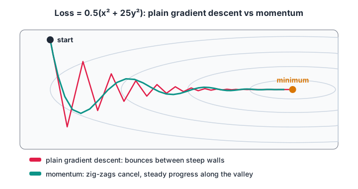
On a long, narrow valley, plain gradient descent wastes steps bouncing between the steep walls. Momentum averages those bounces away and keeps moving along the valley floor.
Quick check
Your training loss jumps to nan after a few steps. What is the most likely first fix?
A learning rate above the stable limit makes the loss grow every step until it overflows. Lowering it is the first thing to try.
Momentum, RMSProp and Adam explained
Momentum
Momentum keeps a running "velocity": v ← β·v + g, then w ← w − lr·v, with β usually 0.9. Gradients that keep pointing the same way add up; gradients that flip sign each step cancel out, so the zig-zag shrinks.
RMSProp
RMSProp tracks a running average of the squared gradient for each weight, then divides the step by its square root. A weight with consistently large gradients gets a smaller step; a weight with tiny gradients gets a larger one. Every parameter gets its own effective learning rate.
Adam
Adam (adaptive moment estimation) combines both ideas. It keeps a momentum-style average m of the gradients and an RMSProp-style average v of the squared gradients, corrects both for starting at zero, and steps by lr · m̂ / (√v̂ + ε).
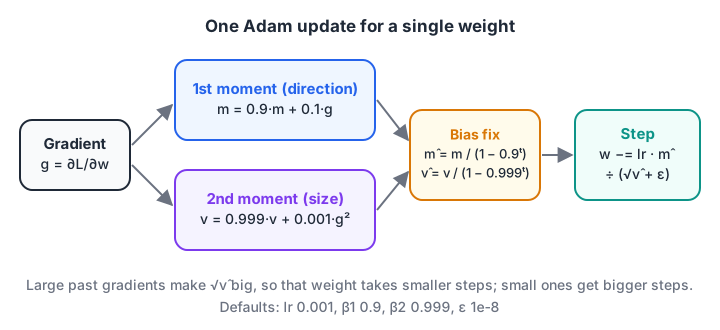
Adam's two running averages. The first gives direction with momentum, the second scales each weight's step by how large its gradients usually are.
Now race them on two surfaces: the narrow valley from before, and a badly scaled one where the flat direction is 2,500 times flatter than the steep one.
import numpy as np

def make(curv):                              # loss = 0.5 * sum(curv * p**2)
    return lambda p: 0.5 * np.sum(curv * p ** 2), lambda p: curv * p

def sgd(p, g, s, t, lr):        return p - lr * g
def momentum(p, g, s, t, lr, beta=0.9):
    s["v"] = beta * s.get("v", 0) + g;   return p - lr * s["v"]
def adam(p, g, s, t, lr, b1=0.9, b2=0.999, eps=1e-8):
    s["m"] = b1 * s.get("m", 0) + (1 - b1) * g
    s["v"] = b2 * s.get("v", 0) + (1 - b2) * g ** 2
    m_hat, v_hat = s["m"] / (1 - b1 ** t), s["v"] / (1 - b2 ** t)
    return p - lr * m_hat / (np.sqrt(v_hat) + eps)

def steps_needed(opt, lr, curv, limit=5000):
    loss, grad = make(curv)
    p, s = np.array([-8.0, 1.5]), {}
    for t in range(1, limit + 1):
        p = opt(p, grad(p), s, t, lr)
        if loss(p) < 1e-4:
            return t
    return f">{limit}"

for label, curv in [("narrow valley (1 vs 25)", np.array([1.0, 25.0])),
                    ("badly scaled (0.01 vs 25)", np.array([0.01, 25.0]))]:
    print(label)
    for name, opt, lr in [("SGD", sgd, 0.035), ("Momentum", momentum, 0.035), ("Adam", adam, 0.3)]:
        print(f"   {name:9s} lr={lr:<6} steps to loss < 1e-4: {steps_needed(opt, lr, curv)}")
On the narrow valley, SGD needs 178 steps while momentum and Adam need about 105 to 111. On the badly scaled surface, plain SGD has not finished after 5,000 steps, momentum needs about 1,100, and Adam finishes in 86. Adam's per-weight scaling makes flat and steep directions look alike, which real networks with millions of unevenly scaled weights need.
Which optimizer should you use?
| Optimizer | Extra memory per weight | Strength | Weakness | Common default |
|---|---|---|---|---|
| SGD | none | Simple, generalises well | Slow on uneven surfaces | lr 0.01 to 0.1 |
| SGD + momentum | 1 value | Smooths zig-zags | Still one global step size | lr 0.01 to 0.1, β 0.9 |
| RMSProp | 1 value | Per-weight step sizes | No momentum on its own | lr 0.001 |
| Adam | 2 values | Fast, little tuning | Can generalise slightly worse | lr 0.001, β (0.9, 0.999) |
| AdamW | 2 values | Adam with proper weight decay | Same as Adam | lr 0.001, weight decay 0.01 |
AdamW fixes one detail of Adam: it applies weight decay directly to the weights rather than mixing it into the gradient average. It is the usual choice for transformers and many modern models. Weight decay itself is the neural-network cousin of the penalty in ridge and lasso regularisation.
Quick check
What does Adam add that momentum alone does not have?
Adam divides each weight's step by the square root of its running squared-gradient average, so steep and flat directions are treated alike.
Learning rate schedules and the PyTorch version
Most training runs also change the learning rate over time. A short warm-up starts small for stability, then a decay such as cosine shrinks the rate so the model settles into a minimum.
Follow these steps for a new model:
- Start with AdamW, learning rate 0.001, batch size 32 to 128.
- Watch the training loss for the first few hundred steps. If it rises or prints
nan, divide the learning rate by 3 or 10. - Add a cosine schedule once the basic run works.
- If you have time and need the best test accuracy, try SGD with momentum 0.9 and a larger rate such as 0.05, as many image models do.
- Tune the rate together with batch size; hyperparameter tuning covers search strategies.
In PyTorch 2.x the whole loop looks like this:
import torch
from torch import nn

model = nn.Sequential(nn.Linear(3, 32), nn.ReLU(), nn.Linear(32, 1))
optimizer = torch.optim.AdamW(model.parameters(), lr=1e-3, weight_decay=0.01)
# alternative: torch.optim.SGD(model.parameters(), lr=0.05, momentum=0.9, nesterov=True)
scheduler = torch.optim.lr_scheduler.CosineAnnealingLR(optimizer, T_max=50)
loss_fn = nn.MSELoss()

for epoch in range(50):
    for xb, yb in train_loader:          # a DataLoader yielding mini-batches
        optimizer.zero_grad()            # clear old gradients
        loss = loss_fn(model(xb), yb)
        loss.backward()                  # backprop fills .grad
        optimizer.step()                 # apply the update rule
    scheduler.step()                     # once per epoch
If you would rather debug loss curves like these with an instructor beside you, Debugshala's ML training with optimiser labs runs at the Old Palasia campus.
Common mistakes with optimizers
- Changing the optimizer before checking the learning rate. A bad rate breaks every optimizer; fix the rate first.
- Forgetting
optimizer.zero_grad(). Gradients accumulate across steps and the updates become huge. - Not shuffling data between epochs. Mini-batches then repeat the same order, and the noise that helps SGD becomes a bias.
- Using Adam's
weight_decayand expecting AdamW behaviour. They are different; pick AdamW when you want decoupled weight decay. - Unscaled input features. Features on wildly different scales create the badly scaled surface from the race above. Standardising inputs, as in data preprocessing and scaling, helps every optimizer.
Key takeaways
- Gradient descent moves weights against the gradient; the optimizer decides the exact step.
- Mini-batches of 32 to 256 give a good balance of speed and accuracy.
- The steepest direction limits the learning rate, which makes plain SGD crawl in flat directions.
- Momentum cancels zig-zags; Adam adds per-weight step sizes and handles badly scaled problems.
- AdamW at 0.001 with a schedule is a strong default.
Next in the series, batch normalisation and dropout make networks easier to optimise and less likely to overfit. To check your understanding, solve gradient and optimiser MCQs on Debugshala Test.
FAQ
What is the difference between SGD and Adam?
SGD moves every weight by the same learning rate times its gradient. Adam keeps two running averages per weight, one of gradients and one of squared gradients, and uses them to give each weight its own step size with momentum. Adam usually converges faster with less tuning; well-tuned SGD sometimes generalises slightly better.
What is a good learning rate for Adam?
0.001 is the standard starting point and the default in PyTorch and Keras. Fine-tuning a pretrained model often uses smaller rates such as 0.00002 to 0.0001. If the loss explodes, divide by 10; if it barely moves after a few hundred steps, try 3 times larger.
What batch size should I use for training a neural network?
Start with 32 to 128 and pick the largest size that fits in memory without hurting accuracy. Larger batches give smoother gradients and better hardware use, but often need a larger learning rate and warm-up. Tiny batches are noisy and slow on GPUs.
Why is it called stochastic gradient descent?
"Stochastic" means random. Each step estimates the gradient from a randomly chosen example or mini-batch instead of the whole dataset, so the estimate is noisy. On average it points the right way, and the randomness can even help the model escape poor regions of the loss surface.
Can I learn optimizers and deep learning at Debugshala in Indore?
Yes. Debugshala's Machine Learning course at its Old Palasia campus in Indore covers training neural networks, including gradient descent and optimizers. Classes run in English and Hindi, fresh graduates and non-IT learners can join, placement assistance is offered, and you can attend a free demo class first.
From the team behind this site
Go further with the Data Science & AI Course at Debugshala
These tutorials are written by Debugshala, a training and placement institute at Old Palasia, Indore. The classroom course adds live mentoring, real projects and interview preparation.
- Offline classes at Old Palasia, Indore
- Free demo class before you pay
- Non-IT, fresher and year-gap friendly
- Placement assistance
700+ students placed · 200+ hiring partners · 4.9★ Google rating
