

Activation Functions in Neural Networks: ReLU, Sigmoid, GELU
Activation functions explained with NumPy: sigmoid, tanh, ReLU, Leaky ReLU, GELU and softmax, their derivatives, vanishing gradients and which one to pick.
Walk into an electrical shop in Siyaganj and ask for a switch for your ceiling fan. The shopkeeper will show you three kinds. A plain on/off switch, a dimmer that turns smoothly from dark to bright, and a regulator with a dead zone at the bottom that does nothing until you turn it past the first notch.
All three take the same input, how far you turn the knob, and give different outputs.
Every neuron in a network has a switch like this. You met one in the NumPy neural network from scratch, where sigmoid turned a weighted sum into a probability. This tutorial looks at the whole shelf of switches and explains why most modern networks no longer pick sigmoid for their hidden layers.
What is an activation function in a neural network?
Map the shop to the network:
- How far you turn the knob is the neuron's pre-activation
z = w·x + b. - The switch is the activation function
f. - The light that reaches the room is the neuron's output
a = f(z), which becomes input to the next layer. - How sensitive the light is to a tiny twist of the knob is the derivative
f'(z). Backpropagation multiplies these derivatives together, so they matter as much as the function itself.
An activation function is a fixed non-linear function applied to each neuron's weighted sum, which lets a neural network represent curved, non-linear relationships and controls how gradients flow back during training.
It has no weights of its own. You pick it per layer, and every neuron in that layer uses it.
Why does a neural network need a non-linear activation?
Suppose you remove the activations and keep two layers: h = W1·x and y = W2·h. Substitute and you get y = (W2·W1)·x. The product W2·W1 is just another matrix. Two layers, ten layers or a hundred layers without activations all shrink to one linear layer.
You can check this in a few lines:
import numpy as np
rng = np.random.default_rng(0)

x = rng.normal(size=(5, 3))               # 5 samples, 3 features
W1 = rng.normal(size=(3, 4))
W2 = rng.normal(size=(4, 2))

deep_linear = (x @ W1) @ W2               # two layers, no activation
W_single = W1 @ W2                        # one merged matrix
print("same output as one layer?", np.allclose(deep_linear, x @ W_single))

relu = lambda z: np.maximum(0, z)
deep_relu = relu(x @ W1) @ W2             # add ReLU in between
print("same with ReLU in between?", np.allclose(deep_relu, x @ W_single))
The first line prints True and the second prints False. The ReLU bends the function, so the second layer now builds on something a single matrix cannot copy. That bend is the whole reason hidden layers add power.
Quick check
What happens if you stack three linear layers with no activation functions?
The product of the weight matrices is just one matrix, so the whole stack is one linear transform.
Common activation functions compared
The four curves below cover most of what you will meet in practice. Look at two things in each: the range of outputs, and where the curve goes flat, because a flat curve means a near-zero derivative.
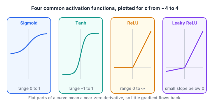
Sigmoid and tanh flatten at both ends, ReLU is flat only for negative inputs, and Leaky ReLU keeps a small slope everywhere.
| Function | Formula | Output range | Derivative | Typical use |
|---|---|---|---|---|
| Sigmoid | 1 / (1 + e^-z) | 0 to 1 | s(1 − s), max 0.25 | Binary output layer |
| Tanh | (e^z − e^-z) / (e^z + e^-z) | −1 to 1 | 1 − t², max 1 | Small RNNs, gates |
| ReLU | max(0, z) | 0 to ∞ | 1 if z > 0 else 0 | Default for hidden layers |
| Leaky ReLU | z if z > 0 else 0.01z | −∞ to ∞ | 1 or 0.01 | When many ReLUs die |
| GELU | z · Φ(z) | about −0.17 to ∞ | smooth, near ReLU's | Transformers, modern MLPs |
| Softmax | e^zi / Σ e^zj | 0 to 1, sums to 1 | Jacobian | Multi-class output layer |
Here they are in NumPy, each with its derivative. The last loop compares every hand-written derivative with a numerical slope, which is the cheapest way to catch a sign or formula error.
import numpy as np
from math import erf, sqrt, pi

def sigmoid(z):  return 1 / (1 + np.exp(-z))
def d_sigmoid(z): s = sigmoid(z); return s * (1 - s)
def d_tanh(z):   return 1 - np.tanh(z) ** 2
def relu(z):     return np.maximum(0, z)
def d_relu(z):   return (z > 0).astype(float)
def leaky(z, a=0.01):   return np.where(z > 0, z, a * z)
def d_leaky(z, a=0.01): return np.where(z > 0, 1.0, a)
Phi = np.vectorize(lambda v: 0.5 * (1 + erf(v / sqrt(2))))
def gelu(z):     return z * Phi(z)
def d_gelu(z):   return Phi(z) + z * np.exp(-z ** 2 / 2) / sqrt(2 * pi)

z = np.array([-3.0, -0.5, 0.7, 2.0])     # avoid z = 0, where ReLU has a kink
pairs = {"sigmoid": (sigmoid, d_sigmoid), "tanh": (np.tanh, d_tanh),
         "relu": (relu, d_relu), "leaky": (leaky, d_leaky), "gelu": (gelu, d_gelu)}
eps = 1e-5
for name, (f, df) in pairs.items():
    numeric = (f(z + eps) - f(z - eps)) / (2 * eps)
    print(f"{name:8s} f(z) = {np.round(f(z), 3)}  max derivative error = {np.abs(numeric - df(z)).max():.1e}")
Every error should be around 1e-10 or smaller. If one of your own formulas shows 1e-1, the derivative is wrong, and your network would train in a strange direction without ever crashing.
Vanishing gradients: why sigmoid fell out of favour
Backpropagation multiplies one activation derivative per layer as it travels from the output back to the first layer. Sigmoid's derivative is never larger than 0.25. Multiply 0.25 by itself ten times and you get about 0.000001. The early layers receive almost no learning signal, so they barely change. This is the vanishing gradient problem.
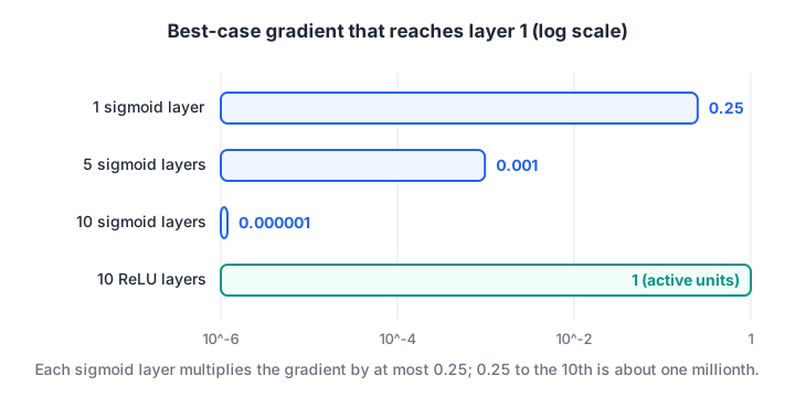
Best case for sigmoid: each layer passes on at most a quarter of the gradient, so ten layers leave about one millionth. Active ReLU units pass the gradient through unchanged.
The simulation below pushes a random input through ten layers and records how big the gradient is when it reaches layer 1. The weights use a sensible starting scale for each activation, so the difference you see comes from the activation itself.
import numpy as np
rng = np.random.default_rng(1)

def grad_at_first_layer(act, d_act, scale, layers=10, width=64):
    a, cache = rng.normal(size=width), []
    for _ in range(layers):
        W = rng.normal(scale=scale / np.sqrt(width), size=(width, width))
        z = W @ a
        cache.append((W, z))
        a = act(z)
    g = np.ones(width)                       # pretend dLoss/dOutput = 1
    for W, z in reversed(cache):
        g = W.T @ (g * d_act(z))
    return np.abs(g).mean()

sig = lambda z: 1 / (1 + np.exp(-z))
print("sigmoid:", f"{grad_at_first_layer(sig, lambda z: sig(z) * (1 - sig(z)), 1.0):.2e}")
print("tanh:   ", f"{grad_at_first_layer(np.tanh, lambda z: 1 - np.tanh(z) ** 2, 1.0):.2e}")
print("relu:   ", f"{grad_at_first_layer(lambda z: np.maximum(0, z), lambda z: (z > 0) * 1.0, np.sqrt(2)):.2e}")
Sigmoid's gradient at layer 1 comes out about ten million times smaller than ReLU's. Tanh sits in between, because its slope can reach 1 near zero. The sqrt(2) scale for ReLU is He initialisation, which balances the half of the units that output zero.
Dying ReLU and how Leaky ReLU fixes it
ReLU has its own failure mode. If a neuron's weighted sum is negative for every training example, its output is always 0 and its derivative is always 0. No gradient ever reaches its weights, so it stays switched off for good. A large learning rate that throws a bias far negative is the usual cause.
import numpy as np
rng = np.random.default_rng(7)

X = rng.normal(size=(1000, 20))            # 1,000 samples, 20 features
W = rng.normal(scale=0.3, size=(20, 50))   # 50 hidden neurons
b = rng.normal(loc=-2.0, size=50)          # biases knocked negative by a bad update

z = X @ W + b
relu_grad = (z > 0)
leaky_grad = np.where(z > 0, 1.0, 0.01)
dead = (relu_grad.sum(axis=0) == 0).sum()
print("ReLU neurons with zero gradient on every sample:", dead, "of 50")
print("Leaky ReLU neurons with zero gradient:", (leaky_grad.sum(axis=0) == 0).sum(), "of 50")
Leaky ReLU gives negative inputs a slope of 0.01 instead of 0, so even a badly placed neuron still gets a faint signal and can climb back. A lower learning rate and careful initialisation also help.
Quick check
Why does sigmoid cause vanishing gradients in deep networks?
Multiplying many numbers below 0.25 drives the gradient for early layers towards zero.
Softmax: the activation for multi-class outputs
Sigmoid works for one yes/no output, as in logistic regression. When a model must choose one of several classes, say sorting a customer complaint into delivery, payment or quality, the output layer uses softmax. It turns a vector of raw scores (logits) into probabilities that add up to 1.
import numpy as np

def softmax(logits):
    shifted = logits - logits.max()        # subtract the max for numerical safety
    e = np.exp(shifted)
    return e / e.sum()

scores = np.array([2.0, 1.0, 0.1])         # delivery, payment, quality
p = softmax(scores)
print("probabilities:", np.round(p, 3), "sum =", p.sum())

big = np.array([1000.0, 999.0, 998.0])
with np.errstate(over="ignore"):
    print("naive exp overflows to:", np.exp(big)[:1])
print("stable softmax:", np.round(softmax(big), 3))
The naive version returns inf, while the shifted one gives a clean answer. Subtracting the maximum does not change the result, because the shift cancels in the division. Frameworks do this for you.
Quick check
Which output activation fits a model that picks one of five product categories?
Softmax turns the five scores into probabilities that sum to 1, one per category.
How do you choose an activation function?
Follow these steps for a new feed-forward network:
- Start every hidden layer with ReLU and He initialisation. It is cheap and trains well.
- If training shows many dead units, switch hidden layers to Leaky ReLU, or try GELU for a smoother curve.
- For the output layer, match the task: sigmoid for one probability, softmax for one-of-many classes, and no activation (linear) for regression.
- Keep tanh and sigmoid for places that need a bounded value, such as the gates inside an LSTM.
In PyTorch the same choices are one line per layer. This snippet targets PyTorch 2.x:
import torch
from torch import nn

model = nn.Sequential(
    nn.Linear(20, 64),
    nn.ReLU(),                      # or nn.LeakyReLU(negative_slope=0.01), nn.GELU()
    nn.Linear(64, 3),               # 3 raw class scores (logits), no softmax here
)
loss_fn = nn.CrossEntropyLoss()     # applies log-softmax internally
logits = model(torch.randn(8, 20))
probs = torch.softmax(logits, dim=1)  # only when you need probabilities to display
Notice there is no softmax before the loss. nn.CrossEntropyLoss expects raw logits, so adding your own softmax applies it twice and slows learning.
If you want to practise these design choices on real datasets with a mentor checking your code, Debugshala's deep learning sessions in Indore cover them inside the Machine Learning course.
Common mistakes with activation functions
- No activation between layers. The network silently becomes linear and underfits curved data.
- Sigmoid in every hidden layer of a deep model. Early layers stop learning because of vanishing gradients.
- Softmax before a loss that already includes it. You get double squashing and weak gradients.
- ReLU on the output of a regression model. It can never predict a negative number, which hurts targets like profit or temperature change.
- Ignoring initialisation. ReLU pairs with He initialisation and tanh with Xavier (Glorot); a mismatched scale can make activations explode or vanish before training starts, a problem batch normalisation also eases.
Key takeaways
- An activation function adds the non-linearity that lets layers build on each other.
- Its derivative controls gradient flow, so always check derivatives when you write them by hand.
- ReLU is the default hidden activation; Leaky ReLU and GELU are good alternatives.
- Sigmoid and tanh saturate and cause vanishing gradients in deep stacks.
- Pick the output activation by task: sigmoid, softmax or none.
The next step is to see exactly how these derivatives are chained together in backpropagation explained step by step. For hands-on revision, practise activation-function MCQs on Debugshala Test.
FAQ
Which activation function is best for hidden layers?
ReLU is the best starting point for most hidden layers because it is fast and does not saturate for positive inputs. If many neurons stop updating, try Leaky ReLU. Large language models and other transformer-style networks commonly use GELU or similar smooth variants instead.
Is softmax an activation function?
Yes. Softmax is an activation function used on the output layer of multi-class classifiers. Unlike ReLU or sigmoid, it looks at the whole vector of scores at once and turns them into probabilities that add up to 1, so one class's probability depends on all the others.
What is the difference between sigmoid and tanh?
Both are S-shaped curves. Sigmoid outputs values from 0 to 1, while tanh outputs from −1 to 1 and is centred on zero. Tanh's steeper slope near zero gives slightly better gradients, which is why it was preferred over sigmoid for hidden layers before ReLU took over.
Why is ReLU not differentiable at zero, and does it matter?
ReLU has a sharp corner at zero, so its derivative is undefined at exactly that point. In practice it does not matter: frameworks simply use 0 (or 1) there, and an input landing on exactly 0.0 is rare. Training works normally.
Can I learn deep learning activation functions at Debugshala in Indore?
Yes. Debugshala's Machine Learning course in Indore covers neural networks, including activations, at the Old Palasia campus, with teaching in English and Hindi. Fresh graduates and non-IT learners are welcome, placement assistance is offered, and you can attend a free demo class before paying.
From the team behind this site
Go further with the Data Science & AI Course at Debugshala
These tutorials are written by Debugshala, a training and placement institute at Old Palasia, Indore. The classroom course adds live mentoring, real projects and interview preparation.
- Offline classes at Old Palasia, Indore
- Free demo class before you pay
- Non-IT, fresher and year-gap friendly
- Placement assistance
700+ students placed · 200+ hiring partners · 4.9★ Google rating
