

Batch Normalization and Dropout Explained with NumPy Code
Batch normalization and dropout explained: forward passes in NumPy, running statistics, inverted dropout scaling, train vs eval mode and PyTorch usage.
Think of a cricket academy in Indore that holds trial matches every Sunday. One week the pitch is green and every score is low; the next week it is flat and every score is high. A coach who compares raw scores across weeks learns nothing. So the coach compares each player with that day's average: "20 runs above today's mean".
The same academy has a second rule. In practice games, a few random players sit out each over. Nobody can rely on the star opener to carry the side, so every player learns to bat, bowl and field. On match day, the full team plays.
The first rule is batch normalisation. The second is dropout. Both are layers you add to a neural network, and both fix problems you will meet as soon as your networks get deeper than the small ones in neural network from scratch.
What is batch normalisation in a neural network?
Map the academy to a layer:
- One Sunday's trial is a mini-batch of training examples.
- The raw scores are the layer's pre-activations, one column per neuron.
- "Runs above today's average, in today's spread" is the normalised value
x̂ = (x − mean) / √(var + ε). - The coach's own preference for how spread out and where to centre the scores is the learned scale γ (gamma) and shift β (beta).
Batch normalisation is a layer that normalises each feature using the mean and variance of the current mini-batch, then applies a learnable scale and shift, so every layer receives inputs on a stable scale during training.
As earlier layers update, their outputs keep shifting, and later layers must keep re-adapting. Batch norm holds each layer's input steady, which allows larger learning rates and makes training less sensitive to initialisation.
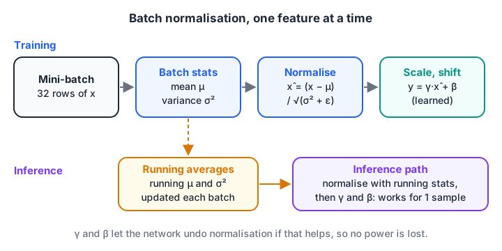
During training, batch norm uses the current batch's statistics and quietly updates running averages. At inference it uses those running averages, so a single input gets a stable answer.
How batch normalisation works, step by step
For each feature (column) in a mini-batch of size m:
- Compute the batch mean
μ = Σx / m. - Compute the batch variance
σ² = Σ(x − μ)² / m. - Normalise:
x̂ = (x − μ) / √(σ² + ε), whereε(about 0.00001) avoids dividing by zero. - Scale and shift:
y = γ · x̂ + β. Gamma and beta are learned by backpropagation like any weight. - Update the running mean and variance with an exponential moving average, for use at inference.
Step 4 matters more than it looks. If forcing mean 0 and variance 1 hurts, the network can learn γ = σ and β = μ and undo the normalisation completely.
Here is a full forward pass in NumPy, with training and inference modes. The three input features sit on wildly different scales, like rupees, ratings and percentages in the same table:
import numpy as np
rng = np.random.default_rng(0)

class BatchNorm1d:
    def __init__(self, features, momentum=0.1, eps=1e-5):
        self.gamma, self.beta = np.ones(features), np.zeros(features)   # learned
        self.run_mean, self.run_var = np.zeros(features), np.ones(features)
        self.momentum, self.eps, self.training = momentum, eps, True

    def __call__(self, x):
        if self.training:
            mean, var = x.mean(axis=0), x.var(axis=0)
            m = self.momentum                                  # update running stats
            self.run_mean = (1 - m) * self.run_mean + m * mean
            self.run_var = (1 - m) * self.run_var + m * var
        else:
            mean, var = self.run_mean, self.run_var
        x_hat = (x - mean) / np.sqrt(var + self.eps)
        return self.gamma * x_hat + self.beta

bn = BatchNorm1d(3)
for step in range(200):                                        # 200 training batches
    batch = rng.normal(loc=[500, -3, 0.6], scale=[100, 0.5, 0.2], size=(32, 3))
    out = bn(batch)
print("batch in  mean/std:", np.round(batch.mean(0), 2), np.round(batch.std(0), 2))
print("batch out mean/std:", np.round(out.mean(0), 2) + 0.0, np.round(out.std(0), 2))
print("running mean      :", np.round(bn.run_mean, 2))
bn.training = False                                            # inference mode
print("eval output for one sample:", np.round(bn(np.array([[600.0, -3.0, 0.6]])), 2))
In training mode every feature leaves with mean 0 and standard deviation 1, whatever its original scale. The running mean has learned roughly [500, −3, 0.6]. In eval mode, the single sample with 600 in the first column comes out near 1.0, "one standard deviation above normal". Without running statistics, a batch of one could not be normalised.
Why batch norm keeps deep networks healthy
The next block pushes a batch through ten ReLU layers whose weights start slightly too small. Without batch norm, the signal fades layer after layer, which is the forward-pass cousin of the vanishing gradients in activation functions. With batch norm, every layer stays on the same scale.
import numpy as np
rng = np.random.default_rng(2)

def normalise(z):                                  # batch norm without gamma/beta
    return (z - z.mean(axis=0)) / np.sqrt(z.var(axis=0) + 1e-5)

x = rng.normal(size=(64, 100))                     # batch of 64, 100 features
for use_bn in [False, True]:
    a, stds = x, []
    for layer in range(10):
        W = rng.normal(scale=0.5 / np.sqrt(100), size=(100, 100))   # slightly too small
        z = normalise(a @ W) if use_bn else a @ W
        a = np.maximum(0, z)
        stds.append(a.std())
    label = "with BN   " if use_bn else "without BN"
    print(label, "activation std at layers 1, 4, 7, 10:", [f"{s:.1e}" for s in stds[::3]])

W = rng.normal(size=(100, 100))
same = np.allclose(normalise(x @ W), normalise(x @ (10 * W)), atol=1e-6)
print("BN output unchanged when all weights are multiplied by 10:", same)
Without batch norm, the activations shrink more than 10,000-fold by layer 10. With it, they hold steady near 0.58. The last line shows a neat side effect: multiplying the weights by 10 changes nothing after normalisation, so a layer's output no longer depends on its weight scale.
Quick check
During inference, what does a batch normalisation layer use to normalise inputs?
Running averages give stable outputs that do not depend on what else is in the batch, so even a single sample works.
What is dropout and why does it reduce overfitting?
In a network, neurons can co-adapt: a group learns to patch each other's mistakes on the training set in a fragile way that fails on new data. Dropout breaks those partnerships, just like benching random players.
Dropout is a regularisation layer that, during training, sets each neuron's output to zero with probability p and scales the survivors by 1 / (1 − p), and does nothing at inference.
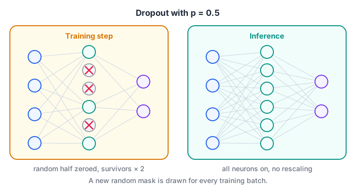
With p = 0.5, each training step uses a different random half of the hidden layer. At inference every neuron is active, and the scaling done during training keeps the expected output the same.
Inverted dropout: why the survivors are scaled up
If 40% of neurons are dropped, the next layer receives only about 60% of its usual total input. At inference, with all neurons on, it would suddenly receive 100%, and its behaviour would shift.
Modern frameworks fix this with inverted dropout: during training they divide the survivors by 0.6, so the expected input is the same in both modes and inference needs no adjustment.
import numpy as np
rng = np.random.default_rng(5)

def dropout(a, p, training):
    if not training or p == 0:
        return a                                   # inference: identity
    mask = rng.random(a.shape) >= p                # keep with probability 1 - p
    return a * mask / (1 - p)                      # inverted dropout scaling

h = rng.uniform(0.5, 1.5, size=(1, 10))            # 10 hidden activations
print("train output:", np.round(dropout(h, 0.4, True), 2))
print("eval output :", np.round(dropout(h, 0.4, False), 2))

big = rng.uniform(0.5, 1.5, size=(10000, 50))
print(f"mean without dropout : {big.mean():.4f}")
print(f"mean with dropout 0.4: {dropout(big, 0.4, True).mean():.4f}")

W = rng.normal(size=(10, 3))                       # dropout as an ensemble average
avg = np.mean([dropout(h, 0.4, True) @ W for _ in range(20000)], axis=0)
print("average of 20,000 thinned networks:", np.round(avg, 2))
print("one full network at inference     :", np.round(h @ W, 2))
The mean activation is almost identical with and without dropout, thanks to the scaling. And the average of 20,000 randomly thinned networks matches the single full network. So dropout also acts like training a huge ensemble of weight-sharing sub-networks and averaging them for free.
Quick check
With dropout p = 0.25 during training, what happens to the neurons that are kept?
Inverted dropout scales the survivors by 1/(1 − p), so no rescaling is needed at inference.
Batch normalisation vs dropout
| Batch normalisation | Dropout | |
|---|---|---|
| Main goal | Stable, faster training | Less overfitting |
| Learned parameters | γ and β per feature | None |
| Training mode | Uses batch mean and variance | Zeros neurons with probability p |
| Inference mode | Uses running mean and variance | Does nothing |
| Sensitive to batch size | Yes, small batches give noisy statistics | No |
| Typical place | After a linear or conv layer, before activation | After the activation, mostly in dense layers |
Dropout belongs to the same family as the weight penalties in ridge and lasso regularisation, and like them, it trades a little training accuracy for better test accuracy. If you are unsure whether you need it, check the train/test gap first, as described in overfitting and the bias-variance trade-off.
For transformers and RNNs, batch statistics are awkward, so those models use layer normalisation, which normalises across the features of each sample instead of across the batch. You will see it inside transformers and attention.
Batch norm and dropout in PyTorch and Keras
This PyTorch 2.x model uses the common Linear, BatchNorm, ReLU, Dropout order:
import torch
from torch import nn

model = nn.Sequential(
    nn.Linear(20, 128),
    nn.BatchNorm1d(128),        # momentum=0.1, eps=1e-5 by default
    nn.ReLU(),
    nn.Dropout(p=0.3),          # p is the probability of zeroing an element
    nn.Linear(128, 2),
)

model.train()                   # batch statistics + random dropout
logits = model(torch.randn(32, 20))

model.eval()                    # running statistics, dropout off
with torch.no_grad():
    prediction = model(torch.randn(1, 20))
In Keras 3 the same layers are keras.layers.BatchNormalization() and keras.layers.Dropout(0.3), and model.fit() and model.predict() switch modes for you. One trap: Keras's momentum=0.99 means "keep 99% of the old running value", while PyTorch's momentum=0.1 means "take 10% from the new batch". They describe the same update from opposite sides.
Getting these modes right is a habit that the neural network modules of Debugshala's machine learning course drill in labs at Old Palasia.
Common mistakes with batch normalisation and dropout
- Forgetting
model.eval()at inference. Dropout keeps zeroing neurons and batch norm uses the test batch's statistics, so predictions change from run to run. - Batch norm with tiny batches. With 2 to 4 samples, the batch mean and variance are noisy. Use layer or group normalisation instead.
- Dropout everywhere at 0.5. Too much dropout causes underfitting. Start at 0.1 to 0.3 and raise it only if the train/test gap stays large.
- Dropping out the output layer. Randomly zeroing the final predictions only adds noise.
- Normalising with stale running statistics. After fine-tuning on very different data, recompute or update the running averages before deploying.
Key takeaways
- Batch norm normalises each feature with batch statistics, then applies learned γ and β.
- It stabilises deep networks, allows larger learning rates and makes layers insensitive to weight scale.
- Dropout randomly zeros neurons in training and acts like an ensemble of thinned networks.
- Both layers switch behaviour between training and inference, so always set the mode.
- Use layer normalisation when batches are small or the model is a transformer.
This completes the Neural Networks section. Next, convolutional neural networks put these layers to work on images. Before moving on, revise regularisation basics with Debugshala Test quizzes.
FAQ
Should batch normalisation go before or after the activation?
The original paper placed it before the activation (Linear, BatchNorm, ReLU), and that remains the most common choice. Placing it after the activation also works and sometimes scores slightly better. Pick one convention and keep it consistent across the network.
Can I use batch normalisation and dropout together?
Yes, but combine them with care. Dropout changes the variance of activations between training and inference, which can disturb batch norm's running statistics when dropout comes right before it. A safe pattern is to put dropout after batch norm and the activation, or to use dropout only in the final dense layers.
What is a good dropout rate?
Between 0.1 and 0.5 for hidden layers. Use 0.1 to 0.3 for convolutional layers or networks with batch norm, and up to 0.5 for large fully connected layers that overfit. Input layers, if dropped at all, use small rates like 0.1. Tune by watching validation accuracy.
Why does my model give different predictions each time?
Usually the model is still in training mode, so dropout is active and batch norm uses batch statistics. Call model.eval() in PyTorch before predicting. In Keras, model.predict() already runs in inference mode.
Where can I learn deep learning techniques like batch norm in Indore?
Debugshala covers neural network training, including batch normalisation and dropout, in its Machine Learning course at the Old Palasia campus in Indore. Teaching is in English and Hindi, fresh graduates and non-IT learners are welcome, placement assistance is available, and you can attend a free demo class before paying.
From the team behind this site
Go further with the Data Science & AI Course at Debugshala
These tutorials are written by Debugshala, a training and placement institute at Old Palasia, Indore. The classroom course adds live mentoring, real projects and interview preparation.
- Offline classes at Old Palasia, Indore
- Free demo class before you pay
- Non-IT, fresher and year-gap friendly
- Placement assistance
700+ students placed · 200+ hiring partners · 4.9★ Google rating
