

Autoencoders Explained: Encoder, Bottleneck and Anomaly Use
Autoencoders explained: train a tiny encoder-decoder in NumPy, compare with PCA, detect anomalies with reconstruction error and meet variational autoencoders.
A tailor on MG Road takes your measurements for a kurta. He does not photograph you from every angle. He writes about eight numbers on a slip: chest, waist, shoulder, length, sleeve and a few more. From that slip, a cutter in the back room rebuilds the whole pattern.
The slip works because bodies are not random. Someone with long arms is usually tall too, so a handful of numbers captures most of what matters. The tailor has, in effect, learned a compressed code for human shapes.
Now imagine a customer wants a costume with one sleeve twice as long as the other. The standard slip has no box for that, and the cutter's pattern comes out wrong. That failure is useful: it tells you this order is unusual.
What is an autoencoder?
Map the tailor's shop to the network:
- You, the customer, are the input
x. - Measuring and writing the slip is the encoder.
- The slip itself is the code, also called the latent representation or bottleneck.
- The cutter rebuilding the pattern is the decoder, producing the reconstruction
x̂. - How far the pattern is from your real shape is the reconstruction error.
An autoencoder is an unsupervised neural network made of an encoder that compresses the input into a low-dimensional code and a decoder that reconstructs the input from that code, trained to make the reconstruction as close to the original as possible.
The target is the input itself, so you need no labels. That makes autoencoders handy when you have plenty of data but nobody has tagged it.
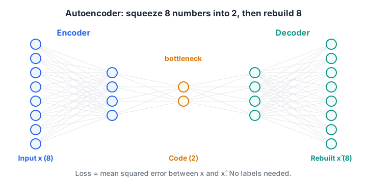
The hourglass shape of an autoencoder. The bottleneck is narrower than the input, so the network cannot simply copy; it must learn which patterns to keep.
How does an autoencoder learn?
Training is the same loop you used in neural network from scratch, with one twist: the target is x itself.
- Encode:
code = f(W1 · x + b1), with fewer outputs than inputs. - Decode:
x̂ = W2 · code + b2, back to the original size. - Loss: mean squared error between
x̂andx. - Backpropagate through decoder and encoder together, then update with an optimiser such as Adam from gradient descent and optimizers.
The bottleneck is what forces learning. If the code were as wide as the input, the network could learn the identity function and copy everything, learning nothing.
Train a tiny autoencoder in NumPy
The data below mimics the tailor's problem: 500 customers, 8 measurements each, all driven by just 2 hidden factors (think height and build) plus a little noise. The autoencoder squeezes 8 numbers into 2 and rebuilds them.
import numpy as np
rng = np.random.default_rng(0)

factors = rng.normal(size=(500, 2))                       # hidden: height, build
mix = rng.normal(size=(2, 8))
X = np.tanh(factors @ mix) + rng.normal(scale=0.05, size=(500, 8))
X = (X - X.mean(0)) / X.std(0)                            # standardise measurements

W1 = rng.normal(scale=0.3, size=(8, 2)); b1 = np.zeros(2)     # encoder: 8 -> 2
W2 = rng.normal(scale=0.3, size=(2, 8)); b2 = np.zeros(8)     # decoder: 2 -> 8
params = [W1, b1, W2, b2]
m = [np.zeros_like(p) for p in params]; v = [np.zeros_like(p) for p in params]
for step in range(1, 1501):
    code = np.tanh(X @ W1 + b1)                  # encode: squeeze to 2 numbers
    X_hat = code @ W2 + b2                       # decode: rebuild 8 numbers
    err = X_hat - X
    d_out = 2 * err / err.size                   # backprop through decoder and encoder
    d_code = (d_out @ W2.T) * (1 - code ** 2)
    grads = [X.T @ d_code, d_code.sum(0), code.T @ d_out, d_out.sum(0)]
    for k, (p, g) in enumerate(zip(params, grads)):   # Adam update
        m[k] = 0.9 * m[k] + 0.1 * g; v[k] = 0.999 * v[k] + 0.001 * g ** 2
        p -= 0.01 * (m[k] / (1 - 0.9 ** step)) / (np.sqrt(v[k] / (1 - 0.999 ** step)) + 1e-8)
    if step in (1, 100, 500, 1500):
        print(f"step {step:4d}  reconstruction MSE {np.mean(err ** 2):.4f}")
print("baseline (predict the average customer): MSE 1.0")
print("first customer's 2-number code:", np.round(code[0], 3))
The error falls from about 0.99 to about 0.04, so 2 numbers rebuild 8 measurements with roughly 96% of the variation explained. Guessing the average customer for everyone gives an error of 1.0, because the data is standardised.
How is an autoencoder different from PCA?
PCA also compresses data into a few numbers, but only with straight-line (linear) projections. In fact, an autoencoder with no activation functions and squared-error loss learns the same subspace as PCA. Add non-linear activations and extra layers, and an autoencoder can follow curved structure that PCA flattens.
| PCA | Autoencoder | |
|---|---|---|
| Mapping | Linear only | Linear or non-linear |
| Training | Closed form, seconds | Gradient descent, needs tuning |
| Interpretability | Components are ranked and orthogonal | Code dimensions have no fixed order |
| Data needed | Works on small data | Needs more data to avoid overfitting |
| Good first choice for | Tabular data, quick reduction | Images, audio, complex sensor data |
Try PCA first. Reach for an autoencoder when PCA's reconstruction is clearly too poor.
Quick check
What is the training target of a basic autoencoder?
An autoencoder learns to reconstruct its own input, so no labels are needed.
Autoencoders for anomaly detection
Back to the costume with mismatched sleeves. An autoencoder trained only on normal data learns to rebuild normal patterns well. Feed it something unusual and the reconstruction is poor. The reconstruction error becomes an anomaly score.
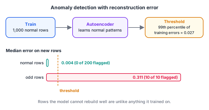
Train on normal rows only, then set a threshold from their errors. New rows whose reconstruction error crosses it are flagged for review.
The steps:
- Train the autoencoder on data you believe is normal.
- Compute the reconstruction error for every training row.
- Set a threshold, for example the 99th percentile of those errors.
- Flag any new row whose error is above the threshold.
import numpy as np
rng = np.random.default_rng(1)

mix = rng.normal(size=(2, 8))
def normal_rows(n):                               # 8 readings driven by 2 hidden factors
    return np.tanh(rng.normal(size=(n, 2)) @ mix) + rng.normal(scale=0.05, size=(n, 8))
X_train, X_new = normal_rows(1000), normal_rows(200)
odd = rng.uniform(-1, 1, size=(10, 8))            # 10 records that break the pattern

P = [rng.normal(scale=0.3, size=(8, 2)), np.zeros(2), rng.normal(scale=0.3, size=(2, 8)), np.zeros(8)]
def rebuild(X):
    code = np.tanh(X @ P[0] + P[1]);  return code, code @ P[2] + P[3]
M = [np.zeros_like(p) for p in P]; V = [np.zeros_like(p) for p in P]
for t in range(1, 1501):                          # same autoencoder + Adam as before
    code, X_hat = rebuild(X_train)
    d_out = 2 * (X_hat - X_train) / X_train.size
    d_code = (d_out @ P[2].T) * (1 - code ** 2)
    for k, g in enumerate([X_train.T @ d_code, d_code.sum(0), code.T @ d_out, d_out.sum(0)]):
        M[k] = 0.9 * M[k] + 0.1 * g;  V[k] = 0.999 * V[k] + 0.001 * g ** 2
        P[k] -= 0.01 * (M[k] / (1 - 0.9 ** t)) / (np.sqrt(V[k] / (1 - 0.999 ** t)) + 1e-8)

score = lambda X: ((X - rebuild(X)[1]) ** 2).mean(axis=1)   # reconstruction error per row
threshold = np.percentile(score(X_train), 99)
print(f"threshold (99th percentile of normal errors): {threshold:.4f}")
print(f"new normal rows flagged: {(score(X_new) > threshold).sum()} of 200")
print(f"odd rows flagged:        {(score(odd) > threshold).sum()} of 10")
print("median error  normal:", round(float(np.median(score(X_new))), 4), " odd:", round(float(np.median(score(odd))), 4))
All 10 odd rows are flagged and none of the 200 new normal rows are. The median error for odd rows is about 75 times higher than for normal ones. Real systems use this idea for card fraud, machine sensor faults and network intrusion, alongside the methods in anomaly detection techniques.
Quick check
In anomaly detection with an autoencoder, which rows get flagged?
The model rebuilds normal patterns well, so unusual rows show up as large reconstruction errors.
Types of autoencoders
- Undercomplete autoencoder: the basic hourglass above, with a code smaller than the input.
- Denoising autoencoder: you add noise to the input but ask it to rebuild the clean original. It learns to remove noise from scans, audio or sensor readings.
- Sparse autoencoder: the code can be wide, but a penalty keeps most code values near zero, so each input activates only a few features.
- Convolutional autoencoder: uses CNN layers in the encoder and transposed convolutions in the decoder, for images.
- Variational autoencoder (VAE): the encoder outputs a distribution instead of a single point, which lets you generate new samples.
Variational autoencoders in one block
A VAE's encoder outputs a mean μ and a log-variance for each code dimension. Training samples a code with the reparameterisation trick, z = μ + σ · ε with random ε, so gradients can still flow through μ and σ.
A KL divergence penalty pulls every code distribution towards a standard normal, which keeps the code space smooth. After training, you sample z from a standard normal and decode it to create new data.
import numpy as np
rng = np.random.default_rng(3)

mu = np.array([0.8, -1.2])            # encoder output for one customer: centre
log_var = np.array([-2.0, -0.5])      # and log-variance (log keeps variance positive)

std = np.exp(0.5 * log_var)
for _ in range(3):                    # reparameterisation trick: z = mu + std * noise
    z = mu + std * rng.normal(size=2)
    print("sampled code z:", np.round(z, 3))

def kl_to_standard_normal(mu, log_var):
    return -0.5 * np.sum(1 + log_var - mu ** 2 - np.exp(log_var))
print(f"KL penalty for this customer : {kl_to_standard_normal(mu, log_var):.3f}")
print(f"KL penalty if mu=0, var=1    : {abs(kl_to_standard_normal(np.zeros(2), np.zeros(2))):.3f}")
print("random code for generation   :", np.round(rng.normal(size=2), 3))
The KL penalty is zero only when the code distribution is exactly a standard normal, so the model balances rebuilding well against keeping codes tidy. VAEs are an ancestor of today's image generators; their adversarial rival is covered in GANs explained.
Building an autoencoder in PyTorch
import torch
from torch import nn

class AutoEncoder(nn.Module):
    def __init__(self, n_features=8, code_size=2):
        super().__init__()
        self.encoder = nn.Sequential(nn.Linear(n_features, 16), nn.ReLU(),
                                     nn.Linear(16, code_size))
        self.decoder = nn.Sequential(nn.Linear(code_size, 16), nn.ReLU(),
                                     nn.Linear(16, n_features))

    def forward(self, x):
        return self.decoder(self.encoder(x))

model = AutoEncoder()
optimizer = torch.optim.Adam(model.parameters(), lr=1e-3)
x = torch.randn(64, 8)                       # a batch of normal rows
loss = nn.functional.mse_loss(model(x), x)   # target is the input itself
optimizer.zero_grad(); loss.backward(); optimizer.step()
Once trained, model.encoder(x) gives you the compressed code for clustering or plotting, and the per-row MSE gives you anomaly scores. To build projects like a fraud detector around this idea with mentors, see an ML course in Indore where you build autoencoders from scratch at Debugshala.
Common mistakes with autoencoders
- A bottleneck that is too wide. The network learns to copy and the code is useless. Shrink it until reconstruction starts to suffer, then back off a little.
- Training on data full of anomalies. The model learns to rebuild them too, and the error stops separating them.
- Unscaled features. One large-valued column dominates the squared error. Standardise first.
- Setting the threshold on test data. Pick it from training or validation errors only.
- Expecting good samples from a plain autoencoder. Random codes decode to junk; use a VAE if you want to generate.
Key takeaways
- An autoencoder = encoder + bottleneck code + decoder, trained to rebuild its input.
- The narrow bottleneck forces it to learn the structure of the data, without labels.
- A linear autoencoder matches PCA; non-linear ones capture curved structure.
- Reconstruction error is a ready-made anomaly score.
- Denoising, sparse, convolutional and variational versions suit different jobs; VAEs can generate.
For more hands-on array work like the code above, test your NumPy reshaping skills on Debugshala Test.
FAQ
Is an autoencoder supervised or unsupervised?
An autoencoder is usually called unsupervised, or more precisely self-supervised. It needs no human labels because the input serves as its own target. The training itself uses the same loss and backpropagation as a supervised network, which is why the "self-supervised" label is common.
What is the bottleneck in an autoencoder?
The bottleneck is the narrowest layer in the middle of the network, holding the compressed code. Its size controls how much the network must compress: too wide and it simply copies the input, too narrow and the reconstruction loses important detail. You choose it by checking reconstruction error.
What is the difference between an autoencoder and a VAE?
A plain autoencoder maps each input to one fixed code. A variational autoencoder maps each input to a probability distribution and adds a KL penalty that keeps the code space smooth and close to a standard normal. That smoothness lets you sample new codes and decode them into realistic new data.
Can autoencoders be used for image compression?
They can learn compact codes for images, and research systems use them for learned compression. Everyday formats like JPEG still dominate because they are fast and standard. In practice, autoencoders are more often used for denoising images, finding defects in product photos and creating features for other models.
Where can I learn autoencoders and deep learning in Indore?
Debugshala's Machine Learning course at the Old Palasia campus in Indore covers neural networks and unsupervised deep learning ideas such as autoencoders. Teaching is in English and Hindi, fresh graduates and non-IT learners can join, placement assistance is offered, and a free demo class is available before you pay.
From the team behind this site
Go further with the Data Science & AI Course at Debugshala
These tutorials are written by Debugshala, a training and placement institute at Old Palasia, Indore. The classroom course adds live mentoring, real projects and interview preparation.
- Offline classes at Old Palasia, Indore
- Free demo class before you pay
- Non-IT, fresher and year-gap friendly
- Placement assistance
700+ students placed · 200+ hiring partners · 4.9★ Google rating
