

GANs Explained: Train a Generative Adversarial Network in NumPy
GANs explained: generator vs discriminator, the minimax and non-saturating losses, a toy 1D GAN trained in NumPy, mode collapse and a PyTorch training loop.
A young cook opens a poha cart near Chappan Dukan and wants his poha to taste exactly like the famous stall down the lane. A regular customer agrees to help. Every morning she gets two plates without labels, one from each stall, and says which one is the original.
At first it is easy: his poha has too much turmeric and no jeeravan. She tells him what gave it away, and he fixes it. Then she notices subtler things, thick sev, sharp lemon, and he fixes those too.
After a few months she is guessing, picking his plate half the time. His poha is now, for her purposes, indistinguishable from the real thing. That contest is a GAN.
What is a GAN?
Map the poha contest to the network:
- The cook is the generator
G. He turns ingredients, plus a little randomness, into a plate. - The randomness each morning is the noise vector
z. - The customer is the discriminator
D. She outputs the probability that a plate is real. - Her feedback is the gradient that flows back into the generator.
- The famous stall's poha is the real data distribution.
A generative adversarial network is a generative model made of two networks trained together in a minimax game: a generator that maps random noise to synthetic samples, and a discriminator that classifies samples as real or fake, so the generator gradually learns to produce data that matches the real distribution.
Unlike autoencoders, a GAN never compares a fake to a specific real example; it learns only from the discriminator's verdict.
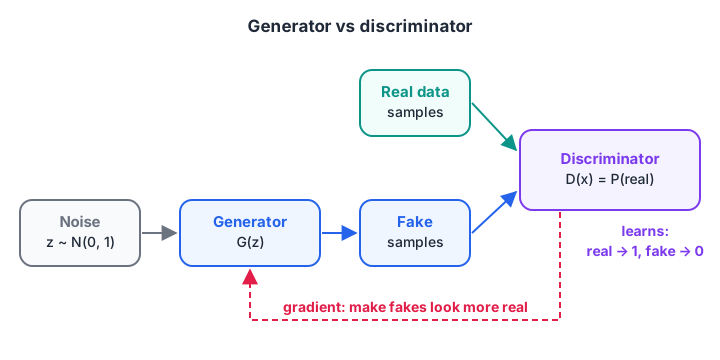
The two players. The discriminator learns from both real and fake samples; the generator learns only through the discriminator's gradient.
How does GAN training work?
The discriminator is a binary classifier with the usual cross-entropy loss. It wants D(real) near 1 and D(fake) near 0. The generator wants the opposite for its fakes. Written as one objective, the game is:
min over G, max over D: E[log D(x_real)] + E[log(1 − D(G(z)))]
In practice, each training step has two parts:
- Train the discriminator. Take a batch of real samples and a batch of fakes from the current generator. Update
Dto classify them correctly. The generator is frozen. - Train the generator. Make a fresh batch of fakes and pass them through
D. Backpropagate the generator's loss through the frozen discriminator intoG's weights, so the fakes look a little more real. - Repeat thousands of times.
Why generators use the non-saturating loss
Early in training, the discriminator easily spots fakes, so D(G(z)) is near 0. The textbook generator loss log(1 − D(G(z))) is almost flat there, so the generator gets almost no gradient when it needs one most. The fix is to minimise −log D(G(z)) instead: same goal, strong gradient when fakes are bad.
import numpy as np

for d_fake in [0.01, 0.1, 0.5, 0.9]:                # how "real" D thinks the fake looks
    s = np.log(d_fake / (1 - d_fake))               # the discriminator's logit
    sat = -d_fake                                   # d/ds of  log(1 - D):  minimax loss
    non_sat = -(1 - d_fake)                         # d/ds of -log D:      non-saturating loss
    print(f"D(fake)={d_fake:4.2f}  logit {s:6.2f}  gradient: minimax {sat:6.3f}   non-saturating {non_sat:6.3f}")
When the discriminator is sure the fake is fake (0.01), the minimax gradient is 0.01 while the non-saturating gradient is 0.99, about 100 times stronger.
Train a toy 1D GAN in NumPy
The mechanics are clearer in one dimension. The "real data" below is the weight of tomatoes per order at a vegetable delivery start-up: about 1.0 kg, with a spread of 0.3 kg. The generator starts by producing plain standard-normal noise.
The two networks are as small as possible while still able to play the game:
- Generator:
G(z) = a·z + b, two weights. It can shift and stretch noise. - Discriminator:
D(x) = sigmoid(w1·x + w2·x² + c). Thex²term lets it notice when the fakes have the wrong spread, not just the wrong centre.
All gradients are written out by hand, using the rules from backpropagation explained.
import numpy as np
rng = np.random.default_rng(0)
sigmoid = lambda s: 1 / (1 + np.exp(-s))

real_batch = lambda n: rng.normal(1.0, 0.3, size=n)   # real data: kg of tomatoes per order
a, b = 1.0, 0.0                                     # generator     G(z) = a*z + b
w1 = w2 = c = 0.0                                   # discriminator D(x) = sigmoid(w1*x + w2*x^2 + c)
D = lambda x: sigmoid(w1 * x + w2 * x ** 2 + c)
lr_d, lr_g, n = 1.0, 0.03, 64

for step in range(1, 1201):
    for _ in range(2):                              # 2 discriminator updates ...
        xr, xf = real_batch(n), a * rng.normal(size=n) + b
        gr, gf = D(xr) - 1, D(xf)                   # gradients of -log D(real) - log(1 - D(fake))
        w1 -= lr_d * (np.mean(gr * xr) + np.mean(gf * xf))
        w2 -= lr_d * (np.mean(gr * xr ** 2) + np.mean(gf * xf ** 2))
        c -= lr_d * (np.mean(gr) + np.mean(gf))
    z = rng.normal(size=n)                          # ... then 1 generator update
    xf = a * z + b
    g_x = (D(xf) - 1) * (w1 + 2 * w2 * xf)          # gradient of -log D(G(z)) for each fake x
    a -= lr_g * np.mean(g_x * z)
    b -= lr_g * np.mean(g_x)
    if step in (1, 100, 300, 600, 1200):
        fake = a * rng.normal(size=5000) + b
        print(f"step {step:4d}: fake mean {fake.mean():.2f}, std {fake.std():.2f} | "
              f"D(real) {D(real_batch(5000)).mean():.2f}, D(fake) {D(fake).mean():.2f}")
print("real data   : mean 1.00, std 0.30")
Read the output as a story:
- Step 1: fakes centre on 0 with spread 1. The discriminator already prefers real samples.
- Step 100: the generator has fixed the centre (about 1.04) but squeezed its spread to about 0.04. Every fake is nearly the same number. This is a tiny version of mode collapse.
- Step 300: the discriminator's
x²term punishes the narrow spread, and the generator overshoots to about 0.44. - Step 600 to 1,200: the swings shrink and the spread settles near 0.32, close to the real 0.30. Both
D(real)andD(fake)hover around 0.5: the customer is guessing.
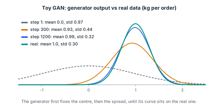
The generator's output distribution at three points in the toy run, against the real distribution. Training ends when the two curves nearly overlap.
The oscillation is not a bug. Each player reacts to the other, so progress comes in swings rather than the smooth slide seen in gradient descent and optimizers.
Quick check
In a well-trained GAN, what does the discriminator output for most samples?
When the generator's distribution matches the real one, the best discriminator is D*(x) = 0.5 everywhere.
Quick check
Your GAN's generator produces the same image for every noise input. What is this called?
Mode collapse is when the generator maps many different noise vectors to one or a few outputs.
What does the discriminator look like at the end?
For any generator, the best possible discriminator has a simple formula: D*(x) = p_real(x) / (p_real(x) + p_fake(x)). Where real data is more common, it leans towards "real", and where fakes are more common, it leans towards "fake".
import numpy as np

def pdf(x, mean, std):                       # normal density
    return np.exp(-0.5 * ((x - mean) / std) ** 2) / (std * np.sqrt(2 * np.pi))

xs = np.array([0.4, 0.7, 1.0, 1.3, 1.6])
for label, g_mean, g_std in [("early generator", 0.0, 1.0),
                             ("collapsed generator", 1.0, 0.05),
                             ("perfect generator", 1.0, 0.3)]:
    p_real, p_fake = pdf(xs, 1.0, 0.3), pdf(xs, g_mean, g_std)
    d_star = p_real / (p_real + p_fake)      # best possible discriminator
    print(f"{label:20s} D*(x) at {xs}: {np.round(d_star, 2)}")
Against the collapsed generator, the best discriminator says "real" everywhere except right at 1.0, where the fakes pile up; that signal pushed the toy generator to widen its spread. Against a perfect generator, it outputs 0.5 everywhere, the theoretical end point of GAN training.
Common GAN problems and fixes
| Problem | What you see | Common fixes |
|---|---|---|
| Mode collapse | Generator outputs only a few kinds of sample | Minibatch statistics in D, Wasserstein loss, more noise dimensions |
| Discriminator wins too easily | D(fake) near 0, generator loss stuck |
Non-saturating loss, lower D learning rate, label smoothing |
| Oscillation | Losses and samples swing without settling | Smaller learning rates, Adam with β1 = 0.5, spectral normalisation |
| No clear stopping point | Losses do not tell you quality | Inspect samples, track a metric such as FID for images |
DCGAN turned these lessons into a recipe for images: convolutional layers, batch normalisation from batch normalisation and dropout, LeakyReLU in the discriminator and Adam with a learning rate of 0.0002 and β1 = 0.5. Later variants such as WGAN, conditional GANs and StyleGAN built on it.
A GAN in PyTorch
This PyTorch 2.x skeleton trains a GAN on 1D data like the toy above. The structure is the same for images; only the two networks change.
import torch
from torch import nn

G = nn.Sequential(nn.Linear(8, 32), nn.ReLU(), nn.Linear(32, 1))         # noise -> sample
D = nn.Sequential(nn.Linear(1, 32), nn.LeakyReLU(0.2), nn.Linear(32, 1))  # sample -> logit
opt_g = torch.optim.Adam(G.parameters(), lr=2e-4, betas=(0.5, 0.999))
opt_d = torch.optim.Adam(D.parameters(), lr=2e-4, betas=(0.5, 0.999))
bce = nn.BCEWithLogitsLoss()

for step in range(5000):
    real = 1.0 + 0.3 * torch.randn(64, 1)
    fake = G(torch.randn(64, 8))

    opt_d.zero_grad()                                  # 1) discriminator step
    loss_d = bce(D(real), torch.ones(64, 1)) + bce(D(fake.detach()), torch.zeros(64, 1))
    loss_d.backward()
    opt_d.step()

    opt_g.zero_grad()                                  # 2) generator step
    loss_g = bce(D(fake), torch.ones(64, 1))           # non-saturating: label fakes as real
    loss_g.backward()
    opt_g.step()
Two details carry the whole algorithm. fake.detach() stops the discriminator's loss from updating the generator. And labelling fakes as "real" (ones) in loss_g is the non-saturating loss from earlier.
Quick check
Why is fake.detach() used in the discriminator update?
detach() cuts the graph, so only the discriminator learns from its own loss in that step.
Where are GANs used, and where have they been replaced?
GANs are used for super-resolution, image-to-image translation (sketch to photo), face filters and synthetic training data. Synthetic samples can help when one class is rare, alongside the methods in handling imbalanced data.
For high-quality text-to-image generation, diffusion models have largely taken over because they train more stably and cover the data more fully. GANs remain popular where speed matters: one generator forward pass makes a sample, while diffusion needs many steps.
To build generative projects like these under guidance, Debugshala's project-led machine learning batches in Indore take you from the NumPy basics to framework code.
Common mistakes when training GANs
- Forgetting
detach()in the discriminator step. The generator then gets updated to help the discriminator, the opposite of its job. - Judging progress by loss alone. GAN losses can look flat while samples improve, or the reverse. Look at samples regularly.
- Letting one network get far stronger. If
D(fake)sits at 0.00 for long, slow the discriminator down. - Using the minimax generator loss directly. It saturates early in training; use the non-saturating form.
Key takeaways
- A GAN pits a generator against a discriminator; neither sees the other's weights, only its outputs.
- Training alternates a discriminator step and a generator step through the frozen discriminator.
- Use the non-saturating generator loss to avoid tiny early gradients.
- Expect oscillation and watch for mode collapse; inspect samples, not just losses.
- The ideal end state is a discriminator outputting 0.5 everywhere.
This closes the Deep Learning series. For a last round of revision, take a final round of ML MCQs on Debugshala Test.
FAQ
What is the difference between a generator and a discriminator?
The generator creates new samples from random noise and tries to make them look real. The discriminator is a classifier that estimates the probability that each sample is real. They train together, each learning from the other's mistakes.
Are GANs supervised or unsupervised?
GANs are usually classed as unsupervised generative models, because they learn from unlabelled data. Internally, the discriminator solves a supervised task with labels it creates itself, real or fake. Conditional GANs add class labels to control what the generator produces.
Why are GANs hard to train?
Two networks chase moving targets, so no single loss goes steadily down. If the discriminator gets too strong, the generator's gradients vanish; if the generator finds one output that fools it, the generator may collapse onto it.
Are GANs still used, or have diffusion models replaced them?
Both are used. Diffusion models dominate high-quality text-to-image generation because they train more stably. GANs remain common for fast, single-step tasks such as super-resolution and real-time filters, and for synthetic tabular or image data.
Can I learn GANs and generative deep learning in Indore?
Debugshala's Machine Learning course at the Old Palasia campus in Indore covers neural networks and deep learning, including generative models. Classes are taught in English and Hindi, fresh graduates and non-IT learners are accepted, placement assistance is offered, and you can attend a free demo class before paying.
From the team behind this site
Go further with the Data Science & AI Course at Debugshala
These tutorials are written by Debugshala, a training and placement institute at Old Palasia, Indore. The classroom course adds live mentoring, real projects and interview preparation.
- Offline classes at Old Palasia, Indore
- Free demo class before you pay
- Non-IT, fresher and year-gap friendly
- Placement assistance
700+ students placed · 200+ hiring partners · 4.9★ Google rating
