

Seaborn Tutorial: Statistical Plots in Python with Examples
A seaborn tutorial for beginners: long-format data, hue, histplot, boxplot, barplot, scatterplot, heatmaps and facets, explained with runnable examples.
Imagine making paneer butter masala two ways. In the first, you roast and grind every spice yourself, measuring each one. In the second, you open a good ready masala mix, add it to the same pan and the same paneer, and adjust the salt at the end.
The ready mix does not replace your kitchen. It saves you twenty minutes on a dish you make often, and you can still add your own touch on top.
What is seaborn?
Mapping the kitchen:
- Grinding every spice by hand is matplotlib: full control, more steps.
- The ready masala mix is seaborn: common statistical charts in one line.
- The same pan and stove are the matplotlib Figure and Axes, which seaborn still draws on.
- Adjusting the salt at the end is calling matplotlib methods such as
ax.set_title()on a seaborn chart.
Seaborn is an open-source Python data visualization library, built on matplotlib, that creates statistical graphics from pandas DataFrames by mapping column names to positions, colours and sizes.
If you have not used matplotlib yet, read data visualization with matplotlib first. Seaborn makes more sense once you know what a Figure and an Axes are.
How does seaborn turn a DataFrame into a chart?
The main idea is that you describe what goes where using column names. Seaborn does the grouping, the maths and the styling.
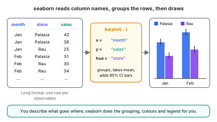
The month column goes to the x-axis, sales to the y-axis and store to colour. Seaborn groups matching rows and draws the mean with an error bar.
Notice that the table has one row per sale record, not one column per store. That is called long format (or tidy data), and seaborn expects it.
Converting wide data to long format
Spreadsheets often arrive in wide format, with one column per category. pd.melt() reshapes them. You can run this:
import pandas as pd

wide = pd.DataFrame({
    "month": ["Jan", "Feb", "Mar"],
    "Palasia": [42, 51, 47],
    "Rau": [25, 32, 29],
})
long = wide.melt(id_vars="month", var_name="store", value_name="sales")
print("Wide:\n", wide, "\n")
print("Long:\n", long)
The wide table has three rows; the long one has six, each with a month, a store and a sales value. Now hue="store" has a column to read. More reshaping tools are in the pandas DataFrame tutorial.
Installing seaborn and setting a theme
pip install seabornSeaborn installs matplotlib, pandas and NumPy if they are missing. The plotting blocks below are display-only on this page because the browser runner cannot open chart windows; copy them into Jupyter or VS Code. Each one builds its own small data, so it needs no internet.
import seaborn as sns
import matplotlib.pyplot as plt

sns.set_theme(style="whitegrid")   # cleaner background for every chart after this
sns.load_dataset() downloads sample datasets such as "tips" from the internet. It is handy for practice, but our examples build data inline so they work offline.
Distribution plots: histplot, kdeplot and boxplot
Distribution plots answer "what values are typical and how spread out are they?" Here are delivery times from two kitchens.
import numpy as np
import pandas as pd
import seaborn as sns
import matplotlib.pyplot as plt

rng = np.random.default_rng(4)
df = pd.DataFrame({
    "minutes": np.concatenate([rng.normal(28, 5, 300), rng.normal(36, 8, 300)]),
    "kitchen": ["Palasia"] * 300 + ["Rau"] * 300,
})
fig, (ax1, ax2) = plt.subplots(1, 2, figsize=(10, 4), layout="constrained")
sns.histplot(data=df, x="minutes", hue="kitchen", kde=True, ax=ax1)
sns.boxplot(data=df, x="kitchen", y="minutes", ax=ax2)
ax2.set_title("Rau is slower and less predictable")
plt.show()
histplot counts values in bins, and kde=True adds a smooth curve estimating the shape. boxplot shows the median as the middle line, the box as the middle 50% of values, and dots as possible outliers.
The box plot numbers are just quartiles, which you can check yourself:
import numpy as np

rng = np.random.default_rng(4)
palasia = rng.normal(28, 5, 300)
rau = rng.normal(36, 8, 300)

for name, x in [("Palasia", palasia), ("Rau", rau)]:
    q1, med, q3 = np.percentile(x, [25, 50, 75])
    iqr = q3 - q1
    outliers = ((x < q1 - 1.5 * iqr) | (x > q3 + 1.5 * iqr)).sum()
    print(f"{name:8} Q1={q1:5.1f} median={med:5.1f} Q3={q3:5.1f} outliers={outliers}")
The 1.5 times IQR rule is what decides which dots a box plot draws beyond the whiskers. It connects directly to outlier detection.
Categorical plots: barplot and countplot
barplot does not just draw your numbers. By default it computes the mean of each group and adds an error bar showing a 95% confidence interval, estimated by bootstrapping (resampling the data many times).
import pandas as pd
import seaborn as sns
import matplotlib.pyplot as plt

df = pd.DataFrame({
    "month": ["Jan"] * 6 + ["Feb"] * 6,
    "store": ["Palasia", "Palasia", "Palasia", "Rau", "Rau", "Rau"] * 2,
    "sales": [42, 38, 44, 25, 28, 22, 51, 47, 55, 30, 34, 31],
})
ax = sns.barplot(data=df, x="month", y="sales", hue="store", errorbar=("ci", 95))
ax.set_ylabel("Average daily sales")
plt.show()
That error bar is not magic. Here is the same bootstrap idea in NumPy for the Palasia January numbers:
import numpy as np

sales = np.array([42, 38, 44])
rng = np.random.default_rng(0)
means = [rng.choice(sales, size=len(sales), replace=True).mean() for _ in range(2000)]
low, high = np.percentile(means, [2.5, 97.5])
print(f"Mean: {sales.mean():.1f}")
print(f"95% bootstrap CI: {low:.1f} to {high:.1f}")
With only three numbers the interval is wide, which is exactly the warning the error bar gives you. If you want to show raw totals instead of means, pass estimator="sum", or use countplot to count rows per category.
Quick check
What does sns.barplot show by default for each group?
barplot uses the mean as its default estimator and adds a bootstrapped 95% confidence interval as the error bar.
Relationship plots and heatmaps
scatterplot and lineplot
scatterplot shows how two numbers relate, and hue, size and style let you add up to three more columns to the same chart.
import numpy as np
import pandas as pd
import seaborn as sns
import matplotlib.pyplot as plt

rng = np.random.default_rng(8)
n = 120
df = pd.DataFrame({"temp_c": rng.uniform(24, 42, n), "weekend": rng.choice(["Yes", "No"], n)})
df["bottles"] = 12 * df["temp_c"] - 180 + np.where(df["weekend"] == "Yes", 60, 0) + rng.normal(0, 20, n)

sns.scatterplot(data=df, x="temp_c", y="bottles", hue="weekend", style="weekend")
plt.show()
lineplot with repeated x values draws the mean line and a shaded confidence band automatically, which is useful for daily readings that repeat across weeks.
heatmap of a correlation matrix
A heatmap colours each cell of a table. The most common use in data science is a correlation matrix during exploratory data analysis. First compute the matrix with pandas (runnable):
import numpy as np
import pandas as pd

rng = np.random.default_rng(2)
temp = rng.uniform(24, 42, 100)
df = pd.DataFrame({
    "temp_c": temp,
    "bottles": 12 * temp + rng.normal(0, 30, 100),
    "umbrellas": 80 - 1.5 * temp + rng.normal(0, 8, 100),
    "price_rs": rng.uniform(18, 22, 100),
})
print(df.corr().round(2))
Then pass the same matrix to seaborn:
import numpy as np
import pandas as pd
import seaborn as sns
import matplotlib.pyplot as plt

rng = np.random.default_rng(2)
temp = rng.uniform(24, 42, 100)
df = pd.DataFrame({
    "temp_c": temp,
    "bottles": 12 * temp + rng.normal(0, 30, 100),
    "umbrellas": 80 - 1.5 * temp + rng.normal(0, 8, 100),
    "price_rs": rng.uniform(18, 22, 100),
})
sns.heatmap(df.corr(), annot=True, fmt=".2f", cmap="vlag", vmin=-1, vmax=1)
plt.show()
Fix vmin=-1, vmax=1 and use a diverging palette such as "vlag", so that zero correlation sits at the neutral middle colour.
Figure-level vs axes-level seaborn functions
Seaborn has two kinds of functions, and mixing them up is the most common source of confusion.
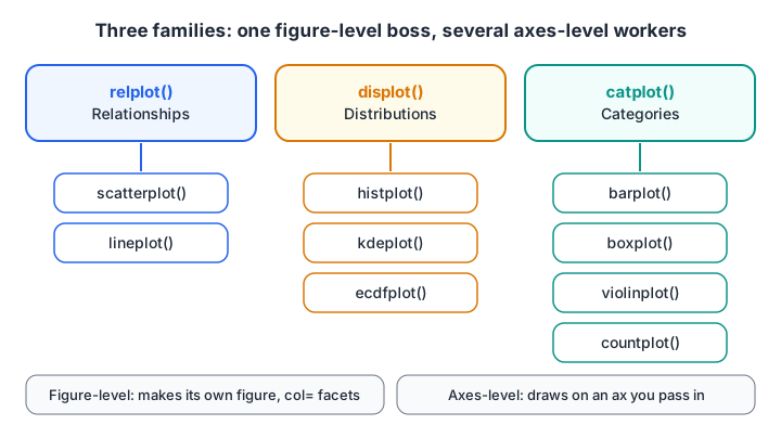
Each figure-level function can draw any of the axes-level plots in its family with the kind argument, and can split the data into facets.
| Axes-level | Figure-level | |
|---|---|---|
| Examples | scatterplot, histplot, boxplot |
relplot, displot, catplot |
| Returns | A matplotlib Axes | A seaborn FacetGrid |
Accepts ax= |
Yes, so it fits into your own subplots | No, it makes its own figure |
Facets with col= and row= |
No | Yes |
| Resize with | figsize on plt.subplots |
height= and aspect= |
Facets are the figure-level superpower: one small chart per category, sharing axes.
import numpy as np
import pandas as pd
import seaborn as sns
import matplotlib.pyplot as plt

rng = np.random.default_rng(4)
df = pd.DataFrame({
    "minutes": np.concatenate([rng.normal(28, 5, 300), rng.normal(36, 8, 300)]),
    "kitchen": ["Palasia"] * 300 + ["Rau"] * 300,
})
g = sns.displot(data=df, x="minutes", col="kitchen", bins=15, height=3.5, aspect=1.2)
g.set_axis_labels("Delivery time (minutes)", "Orders")
plt.show()
The full list of functions and options is in the official seaborn documentation. If you would like feedback on plots like these from a teacher, the Data Science & AI course in Indore by Debugshala uses them throughout its EDA projects.
Quick check
You want one histogram per kitchen, side by side, in a single call. Which function fits?
Figure-level functions like displot can split data into facets with col= and row=.
Common seaborn mistakes
- Passing wide data and expecting hue to work. Melt to long format first.
- Reading a barplot as totals. It shows means with confidence intervals unless you change
estimator. - Passing
ax=to a figure-level function. Use the axes-level version when you build your own subplots. - Using
figsizewithdisplotorcatplot. Setheightandaspectinstead. - Default heatmap colour limits. Without
vminandvmax, a weak correlation can look as strong as a perfect one.
Quick check
Ready to apply these on real data? The next step in the series is data science projects for beginners, and you can warm up with quick pandas and statistics MCQs on Debugshala Test.
Key takeaways
- Seaborn draws statistical charts from DataFrames using column names for
x,yandhue. - It expects long-format data; use
pd.melt()to convert wide tables. - Distribution, categorical and relationship plots cover most EDA needs.
barplotshows means with confidence intervals;boxplotshows quartiles and outliers.- Axes-level functions fit your own subplots; figure-level functions create facets.
FAQ
What is seaborn used for in Python?
Seaborn is used to draw statistical charts quickly from pandas DataFrames, such as histograms, box plots, bar plots with confidence intervals, scatter plots coloured by category, correlation heatmaps and faceted grids. Data scientists mostly use it during exploratory data analysis to spot patterns and outliers.
Should I learn matplotlib or seaborn first?
Learn the basics of matplotlib first, mainly Figure, Axes and labels, and then move to seaborn. Seaborn draws on matplotlib, so you will still use matplotlib methods to adjust titles, limits and saving. A few days of matplotlib basics is enough before starting seaborn.
Why does my seaborn hue not work?
Usually because your data is in wide format, with one column per category, so there is no single column to pass to hue. Convert it with pd.melt() so that the category becomes its own column, then pass that column name to hue.
How do I change the size of a seaborn plot?
For axes-level functions, create the figure first with fig, ax = plt.subplots(figsize=(8, 4)) and pass ax=ax. For figure-level functions such as displot or catplot, use the height and aspect arguments, because they create their own figure.
Where can I learn seaborn and EDA in Indore?
Debugshala covers seaborn, matplotlib and exploratory data analysis in its Data Science & AI course, taught at the Old Palasia campus in Indore and online, in English and Hindi. Non-IT graduates can join, and a free demo class is available before you pay anything.
From the team behind this site
Go further with the Data Science & AI Course at Debugshala
These tutorials are written by Debugshala, a training and placement institute at Old Palasia, Indore. The classroom course adds live mentoring, real projects and interview preparation.
- Offline classes at Old Palasia, Indore
- Free demo class before you pay
- Non-IT, fresher and year-gap friendly
- Placement assistance
700+ students placed · 200+ hiring partners · 4.9★ Google rating
